1. Unit 7. Analyses of LR Production and Costs as Functions of Output

2. Palladium is a Car Maker’s Best Friend? Palladium is a precious metal used as an input in the production of automobile catalytic converters, which are necessary to help automakers meet governmental, mandated environmental standards for removing pollutants from automobile exhaust systems. Between 1992 and 2000, palladium prices increased from about $80 to over $750 per ounce. One response at Ford was a managerial decision to guard against future palladium price increases by stockpiling the metal. Some analysts estimate that Ford ultimately stockpiled over 2 million ounces of palladium and, in some cases, at prices exceeding $1,000 per ounce. Was this a good managerial move?

3. This Little Piggy Wants to Eat Assume Kent Feeds is producing swine feed that has a minimal protein content (%) requirement. Two alternative sources of protein can be used and are regarded as perfect substitutes. What does this mean and what are the implications for what inputs Kent Feeds is likely to use to produce their feed?

4. How Big of a Plant (i.e. K) Do We Want? Assume a LR production process utilizing capital (K) and labor (L) can be represented by a production function Q = 10K 1/2 L 1/2. If the per unit cost of capital is $40 and the per unit cost of L is $100, what is the cost-minimizing combination of K and L to use to produce 40 units of output? 100 units of output? If the firm uses 5 units of K and 3.2 units of L to produce 40 units of output, how much above minimum are total production costs?

5. Q to Produce at Each Location? Funky Foods has two production facilities. One in Dairyland was built 10 years ago and the other in Boondocks was built just last year. The newer plant is more mechanized meaning it has higher fixed costs, but lower variable costs (including labor). What would be your recommendation to management of Funky Foods regarding 1) total product to produce and 2) the quantities to produce at each plant?

6. LR  Max  1.Produce Q where MR = MC 2.Minimize cost of producing Q  optimal input combination

7. Isoquant The combinations of inputs (K, L) that yield the producer the same level of output. The shape of an isoquant reflects the ease with which a producer can substitute among inputs while maintaining the same level of output.

8. Typical Isoquant

9. SR Production in LR Diagram

11. MRTS and MP MRTS= marginal rate of technical substitution = the rate at which a firm must substitute one input for another in order to keep production at a given level = - slope of isoquant = = the rate at which capital can be exchanged for 1 more (or less) unit of labor MP K = the marginal product of K = MP L = the marginal product of L =  Q= MP K  K + MP L  L  Q= 0 along a given isosquant  MP K  K + MP L  L = 0  = ‘inverse’ MP ratio

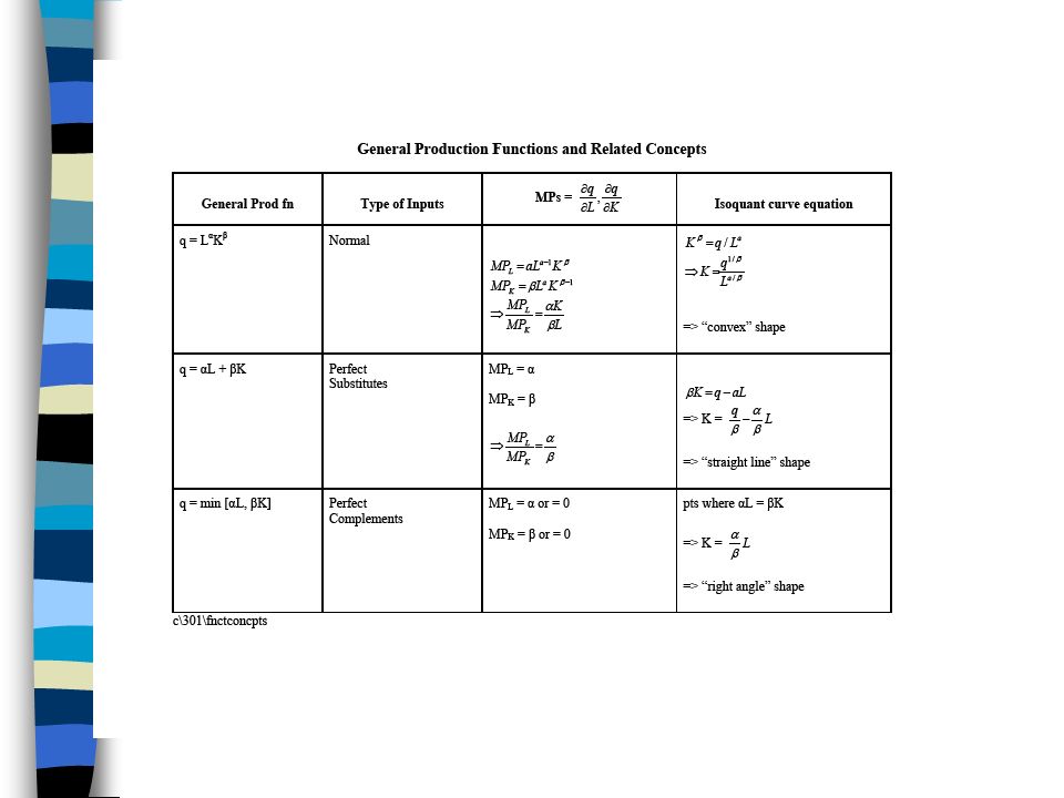
12. Indifference Curve & Isoquant Slopes Indiff CurveIsosquant - slope = MRS = rate at which consumer is willing to exch Y for 1X in order to hold U constant = inverse MU ratio = MU X /MU Y For given indiff curve, dU = 0 Derived from diff types of U fns: 1) Cobb Douglas  U = X  Y  2) Perfect substitutes  U=  X+  Y 3) Perfect complements  U = min [  X,  Y] - slope = MRTS = rate at which producer is able to exch K for 1L in order to hold Q constant = inverse MP ratio = MP L /MP K For given isoquant, dQ = 0 Derived from diff types of production fns: 1) Cobb Douglas  Q = L  K  2) Perfect substitutes  Q=  L+  K 3) Perfect complements  Q = min [  X,  Y]

14. Cobb-Douglas Isoquants Inputs are not perfectly substitutable Diminishing marginal rate of technical substitution Most production processes have isoquants of this shape

15. Linear Isoquants Capital and labor are perfect substitutes

16. Leontief Isoquants Capital and labor are perfect complements Capital and labor are used in fixed- proportions

17. Deriving Isoquant Equation Plug desired Q of output into production function and solve for K as a function of L. Example #1 – Cobb Douglas isoquants –Desired Q = 100 –Production fn: Q = 10K 1/2 L 1/2 –=> 100 = 10K 1/2 L 1/2 –=> K = 100/L (or K = 100L -1 ) –=> slope = -100 / L 2 Exam #2 – Linear isoquants –Desired Q = 100 –Production fn: Q = 4K + L –=> 100 = 4K + L –K = 25 -.25L –=> slope = -.25

18. Budget Line =maximum combinations of 2 goods that can be bought given one’s income =combinations of 2 goods whose cost equals one’s income

19. Isocost Line =maximum combinations of 2 inputs that can be purchased given a production ‘budget’ (cost level) =combinations of 2 inputs that are equal in cost

20. Isocost Line Equation TC 1 = rK + wL  rK = TC 1 – wL  K = Note: slope = ‘inverse’ input price ratio = = rate at which capital can be exchanged for 1 unit of labor, while holding costs constant.

21. Increasing Isocost

22. Changing Input Prices

23. Different Ways (Costs) of Producing q 1

24. Cost Minimization (graph)

25. LR Cost Min (math)  - slope of isoquant = - slope of isocost line     

26. Reducing LR Cost (e.g.)

27. SR vs LR Production

30. Assume a production process: Q=10K 1/2 L 1/2 Q=units of output K=units of capital L=units of labor R=rental rate for K = $40 W=wage rate for L = $10

31. Given q = 10K 1/2 L 1/2 QKLTC=40K+10L 40*2*8*160* 100*5*20*400* 4053.2232 100250580 *  LR optimum for given q

32. Given q = 10K 1/2 L 1/2, w=10, r=40 Minimum LR Cost Condition  inverse MP ratio = inverse input P ratio  (MP of L)/(MP of K) = w/r  (5K 1/2 L -1/2 )/(5K -1/2 L 1/2 ) = 10/40  K/L = ¼  L = 4K

33. Optimal K for q = 40? (Given L* = 4K*) q = 40 = 10K 1/2 L 1/2  40 = 10 K 1/2 (4K) 1/2  40 = 20K  K* = 2  L* = 8  min SR TC = 40K* + 10L* = 40(2) + 10(8) = 80 + 80 = $160

34. SR TC for q = 40? (If K = 5) q = 40 = 10K 1/2 L 1/2  40 = 10 (5) 1/2 (L) 1/2  L = 16/5 = 3.2  SR TC = 40K + 10L = 40(5) + 10(3.2) = 200 + 32 = $232

35. Optimal K for q = 100? (Given L* = 4K*) Q=100 = 10K 1/2 L 1/2  100 = 10 K 1/2 (4K) 1/2  100 = 20K  K* = 5  L* = 20  min SR TC = 40K* + 10L* = 40(5) + 10(20) = 200 + 200 = $400

36. SR TC for q = 100? (If K = 2) Q = 100 = 10K 1/2 L 1/2  100 = 10 (2) 1/2 (L) 1/2  L = 100/2 = 50  SR TC = 40K + 10L = 40(2) + 10(50) = 80 + 500 = $580

37. Two Different costs of q = 100

38. LRTC Equation Derivation [i.e. LRTC=f(q)]  LRTC = rk* + wL* = r(k* as fn of q) + w(L* as fn of q) To find K* as fn q from equal-slopes condition L*=f(k), sub f(k) for L into production fn and solve for k* as fn q To find L* as fn q from equal-slopes condition L*=f(k), sub k* as fn of q for f(k) deriving L* as fn q

39. LRTC Calculation Example Assumeq = 10K 1/2 L 1/2, r = 40, w = 10 L* = 4K (equal-slopes condition)  K* as fn q  q= 10K 1/2 (4K) 1/2 = 10K 1/2 2K 1/2 = 20K   L* as fn q  L*= 4K* = 4(.05 q) L*=.2q  LR TC = rk* + wL* = 40(.05q)+10(.2q) = 2q + 2q = 4q

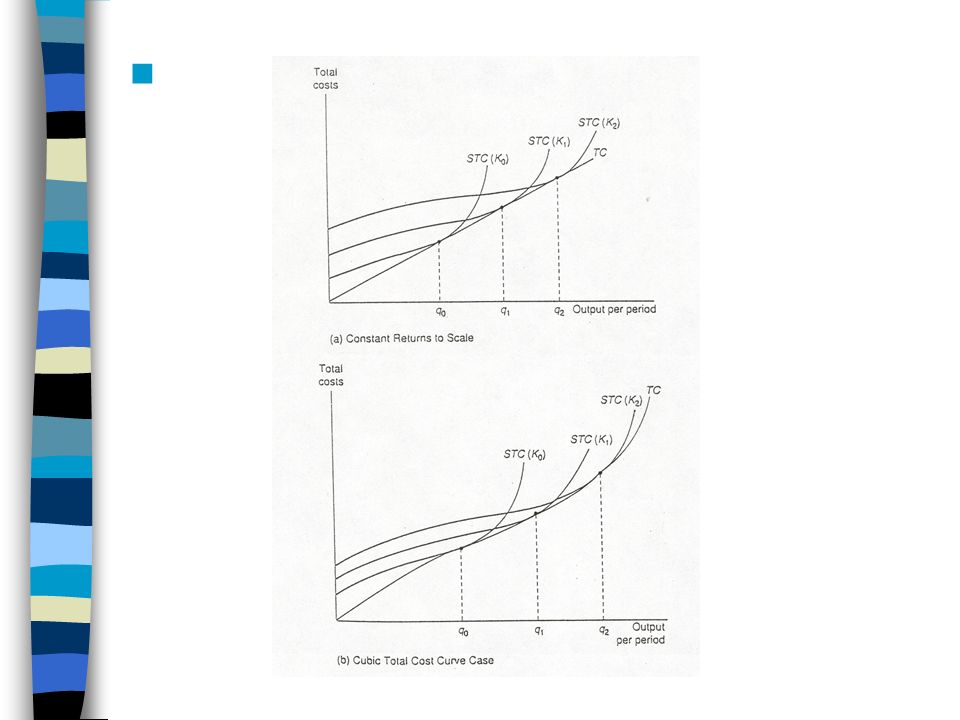
40. Graph of SRTC and LRTC

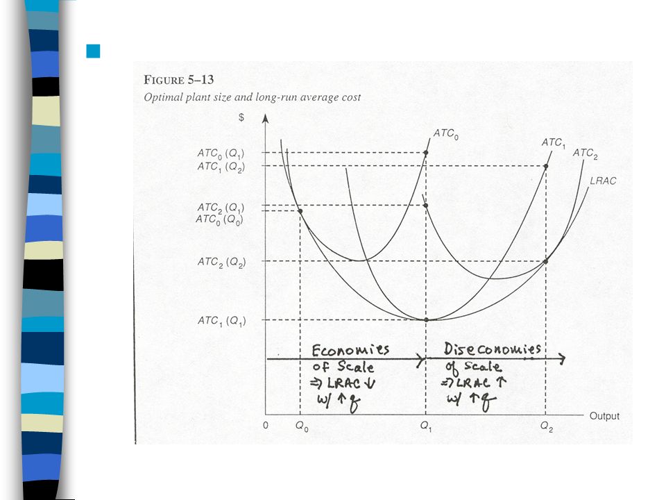
41. Optimal* Size Plant (i.e. K) (*=> to min TC of q 1 ) StepExample 1. Solve SR prod. fn. for L = f(q, ) 2. Set up TC as fn of K (given q, r, w) 3. Min TC w.r.t.

42. Expansion Path  LRTC

43. 

44. Technological Progress

45. Returns to Scale  a LR production concept that looks at how the output of a business changes when ALL inputs are changed by the same proportion (i.e. the ‘scale’ of the business changes) Let q 1 = f(L,K) = initial output q 2 = f(mL, mK) = new output m = new input level as proportion of old input level Types of Returns to Scale: 1) Increasing  q 2 > mq 1 2) Constant  q 2 = mq 1 3) Decreasing  q 2 < mq 1  output ↑ < input ↑

47. Assume a firm is considering using two different plants (A and B) with the corresponding short run TC curves given in the diagram below. $ Q1Q1 Q of output TC A TC B Explain: 1.Which plant should the firm build if neither plant has been built yet? 2.How do long-run plant construction decisions made today determine future short-run plant production costs? 3.How should the firm allocate its production to the above plants if both plants are up and operating?

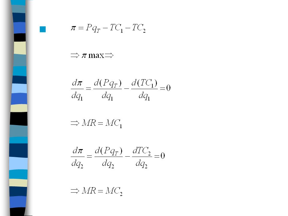
48. Multiplant Production Strategy Assume: P=output price = 70 -.5q T q T =total output (= q 1 +q 2 ) q 1 =output from plant #1 q 2 =output from plant #2  MR = 70 – (q 1 +q 2 ) TC 1 =100+1.5(q 1 ) 2  MC 1 = 3q 1 TC 2 =300+.5(q 2 ) 2  MC 2 = q 2

50. Multiplant  Max (#1) MR = MC 1 (#2) MR = MC 2 (#1) 70 – (q 1 + q 2 ) = 3q 1 (#2) 70 – (q 1 + q 2 ) = q 2 from (#1), q 2 = 70 – 4q 1 Sub into (#2),  70 – (q 1 + 70 – 4q 1 ) = 70 – 4q 1  7q 1 = 70  q 1 = 10, q 2 = 30  = TR – TC 1 – TC 2 = (50)(40) - [100 + 1.5(10) 2 ] - [300 +.5(30) 2 ] = 2000 – 250 – 750 = $1000

51.  If q 1 = q 2 = 20?  =TR -TC 1 -TC 2 = (50)(40) - [100 + 1.5(20) 2 ] - [300 +.5(20) 2 ] = 2000 – 700 – 500 = $800

52. Multi Plant Profit Max (alternative solution procedure) 1.Solve for MC T as fn of q T knowing cost min  MC 1 =MC 2 =MC T  MC 1 =3q 1  q 1 = 1/3 - MC 1 = 1/3 MC T MC 2 = q 2 q 2 = MC 2 = MC T  q 1 +q 2 = q T = 4/3 MC T  MC T = ¾ q T 2.Solve for profit-max q T  MR=MC T  70-q T = ¾ q T  7/4 q T = 70  q* T = 40  MC* T = ¾ (40) = 30

53. Multi Plant Profit Max (alternative solution procedure) 3.Solve for q* 1 where MC 1 = MC* T  3q 1 = 30  q* 1 = 10 4.Solve for q* 2 where MC 2 = MC* T  q* 2 = 30