1. Topological Data Analysis
Applications II
Isabel K. Darcy
Mathematics Department
Applied Mathematical and
Computational Sciences (AMCS)
University of Iowa
This work was partially supported by  the Joint DMS/NIGMS Initiative to Support Research in the Area of Mathematical Biology (NSF ).

3. Create your own homology
3 ingredients:
1.) Objects
2.) Grading
3.) Boundary map

4. Building blocks for a simplicial homology
0-simplex = vertex = v
1-simplex = edge e v1 v2
2-simplex = triangle v2 e2 e1 e3 v1 v3
The building blocks for a simplicial complex consist of zero simplices which are zero dimensional vertices, one simplices which are one-dimensional edges, and 2-simplices which are two dimensional triangles,

5. Grading Grading: Each object is assigned a unique grade
Grading = Partition of R[x]
Ex: Grade = dimension
Grade 0: 0-simplex = vertex = v e v1 v2
Grade 1: 1-simplex = edge = {v1, v2} v2
Grade 2: 2-simplex = triangle = {v1, v2, v3} e1 e2 v1 v3 e3

6. Boundary Map n : Cn  Cn-1 such that 2 = 0   0   0 e v1 v2 v1 v2
 0 e v1 v2 v1 v2 v2 e2 e1 e3 v1 v3 v2 e2 e1 e3 v1 v3 
 0

7. n+1 n 2 1
Cn+1  Cn  Cn-1 . . .  C2  C1  C0  0 n
n+1
Hn = Zn/Bn = (kernel of )/ (image of )
cycles
boundaries = v2 e2 e1 e3 v1 v3

8. ( ) Čech homology Given U Va where Va open for all a in A.
Objects = finite intersections = { Va : ai in A }
Grading = n = depth of intersection.
( Va ) = S Va
Ex: (Va) = 0, (Va Vb) = Va + Vb
(Va Vb Vg) = (Va Vb) + (Va Vg) + (Vb Vg)
a in A U
i = 1 n i
( )
j = 1 n U
i = 1 n U
i = 1
i ≠ j n
n+1 i i 1 U 2 U U U U U

9. Your name homology 3 ingredients: 1.) Objects 2.) Grading
3.) Boundary map
n : Cn  Cn-1 such that = 0

10. Creating a simplicial complex from Data
data points.
In this very simplified case my data points lie in a two-dimensional plane. Normally data points are high dimensional.
For example, I may be comparing the expression or thousands of genes in tumor cells to healthy cells using microarray data. OR I might be comparing politicians voting records. Or I might be comparing the stats of basketball players. These three applications were all, by the way, published by Lum et al this past February in Nature’s Scientific Reports. I have included a link to their paper on my youtube site.
Step 0.) Start by adding data points
= 0-dimensional vertices (0-simplices)

11. Creating a simplicial complex from Data
Recall that to create a simplicial complex, we start by adding 0-simplices (ie 0-dimensional vertices). So our step zero will be to add 0-simplices, but in this case our 0-dimensional points will be
Step 0.) Start by adding 0-dimensional vertices
(0-simplices)

12. Creating a simplicial complex from Data
since my very simple data is 2-dimensional, each point could represent an ordered pair of numbers. For example,
0.) Start by adding 0-dimensional data points
Note: we only need a definition of closeness between data points. The data points do not need to be actual points in Rn

13. Creating a simplicial complex from Data
(1, 8)
(2, 7)
(1, 5)
The points (1, 5), (1, 8), (2, 7). These points could represent actual locations OR each coordinate could represent a particular property. For example, if each point represents a different tumor cell, the first coordinate could represent the gene expression level of the gene coding for the protein ubiquitin hydrolase, while the 2nd coordinate could represent the gene expression level of a different gene. Normally one models thousands of genes at once, Thus each point would have thousands of coordinates where each coordinate represents the expression level of a single gene.
The data points do not need to be described by numbers. Often data is described by numbers but not always.
0.) Start by adding 0-dimensional data points
Note: we only need a definition of closeness between data points. The data points do not need to be actual points in Rn

14. Creating a simplicial complex from Data
(dog, happy)
(wolf, mirthful)
(dog, content)
For example, we could be descriptions. The data can be in just about any format as long as we have a definition of closeness between the data points.
0.) Start by adding 0-dimensional data points
Note: we only need a definition of closeness between data points. The data points do not need to be actual points in Rn

15. Creating a simplicial complex from Data
If two points are “close” , we connect them with an edge
I put quotes around close because we don’t have to use the standard Euclidean distance. Any idea of closeness that is relevant to your application will do. For example correlation is often used. We don’t even need an exact distance or an exact definition of distance, we just need to know when to connect 2 points with an edge.
The definition of closeness will depend upon the application. For now let’s assume standard Euclidean distance.
1.) Adding 1-dimensional edges (1-simplices)
Add an edge between data points that are “close”

16. Creating a simplicial complex from Data
So we can measure (or calculate) the distance between two points to determine if they are “close”. But we still need to define close.
1.) Adding 1-dimensional edges (1-simplices)
Add an edge between data points that are “close”

17. Creating a simplicial complex from Data
So we will connect every pair of vertices if their distance is less than 1.8 cm. If the center of these points represent the 0-dimensional vertices, then this distance is less than our threshold, so we add an edge. Similarly this pair of points satisfy our definition of close, so we add an edge
The distance between this pair of vertices is greater than 1.8, so we won’t connect them with an edge. Continuing to add edges between vertices whenever their distance is less than our threshold of 1.8cm, we now have
1.) Adding 1-dimensional edges (1-simplices)
Let T = Threshold =
Connect vertices v and w with an edge iff
the distance between v and w is less than T

18. Creating a simplicial complex from Data
a one dimensional simplicial complex. Note that we have clustered our data into five disjoint connected sets. So this is one way to cluster our data – that is grouping our data points into disjoint sets based on some definition of similarity. In this case, we have 5 clusters.
We can now add higher dimensional simplices.
1.) Adding 1-dimensional edges (1-simplices)
Add an edge between data points that are “close”

19. Creating a simplicial complex from Data
a one dimensional simplicial complex. Note that we have clustered our data into five disjoint connected sets. So this is one way to cluster our data – that is grouping our data points into disjoint sets based on some definition of similarity. In this case, we have 5 clusters.
We can now add higher dimensional simplices.
1.) Adding 1-dimensional edges (1-simplices)
Add an edge between data points that are “close”

20. Creating the Vietoris Rips simplicial complex
Thus we now have the Vietoris Rips simplicial complex. Note we get the same simplex by adding one dimension at a time
2.) Add all possible simplices of dimensional > 1.

21. Creating the Vietoris Rips simplicial complex
We start again by adding our 0-simplices, our data points. I can indicate the threshold using a ball centered at my data point. The diameter of the ball will be my threshold, so if two balls intersect then the distance between the vertices is less than the threshold, so we connect the pair of vertices with an edge if and only if the balls intersect, so we can get edges after which we can then add all possible higher dimensional simplices.
Note how I grew my balls. As the diameter increases, my threshold which is equal to my diameter increases.
0.) Start by adding 0-dimensional data points
Note: we only need a definition of closeness between data points. The data points do not need to be actual points in Rn

22. H0 counts clusters
a one dimensional simplicial complex. Note that we have clustered our data into five disjoint connected sets. So this is one way to cluster our data – that is grouping our data points into disjoint sets based on some definition of similarity. In this case, we have 5 clusters.
We can now add higher dimensional simplices.

23. H0 counts clusters
a one dimensional simplicial complex. Note that we have clustered our data into five disjoint connected sets. So this is one way to cluster our data – that is grouping our data points into disjoint sets based on some definition of similarity. In this case, we have 5 clusters.
We can now add higher dimensional simplices.

24. Creating the Vietoris Rips simplicial complex
We can compute the number of clusters for a variety of diameters.
We start with 17 data points, so if the diameter is 0, we have 17 clusters. Increasing the diameter, these 2 balls intersect so I now have 16 clusters.
If we continue to increase the diameter, we will eventually create the complex we saw before with 5 clusters, etc until we only have one cluster left.
Eventually this entire page will be purple, but right now, we know have one component.
To choose the threshold, one can determine how long a particular number of clusters lasts, for example for what set of radii do we have five clusters. If we have five clusters for the largest set of radii, then have gives us a good idea where to set the threshold and which simplicial complex best models our data.
I have put links to better animations on my on my YouTube site which may better illustrate this persistence concept. Next month, we will also talk much more about persistence during the live lectures for this course. This is just a preliminary introduction.
0.) Start by adding 0-dimensional data points
Note: we only need a definition of closeness between data points. The data points do not need to be actual points in Rn

25. Cycles
Time
Instead of growing balls, we have a growing path (along with the cover of the path)

26. Creating the Vietoris Rips simplicial complex
We can compute the number of clusters for a variety of diameters.
We start with 17 data points, so if the diameter is 0, we have 17 clusters. Increasing the diameter, these 2 balls intersect so I now have 16 clusters.
If we continue to increase the diameter, we will eventually create the complex we saw before with 5 clusters, etc until we only have one cluster left.
Eventually this entire page will be purple, but right now, we know have one component.
To choose the threshold, one can determine how long a particular number of clusters lasts, for example for what set of radii do we have five clusters. If we have five clusters for the largest set of radii, then have gives us a good idea where to set the threshold and which simplicial complex best models our data.
I have put links to better animations on my on my YouTube site which may better illustrate this persistence concept. Next month, we will also talk much more about persistence during the live lectures for this course. This is just a preliminary introduction.
0.) Start by adding 0-dimensional data points
Note: we only need a definition of closeness between data points. The data points do not need to be actual points in Rn

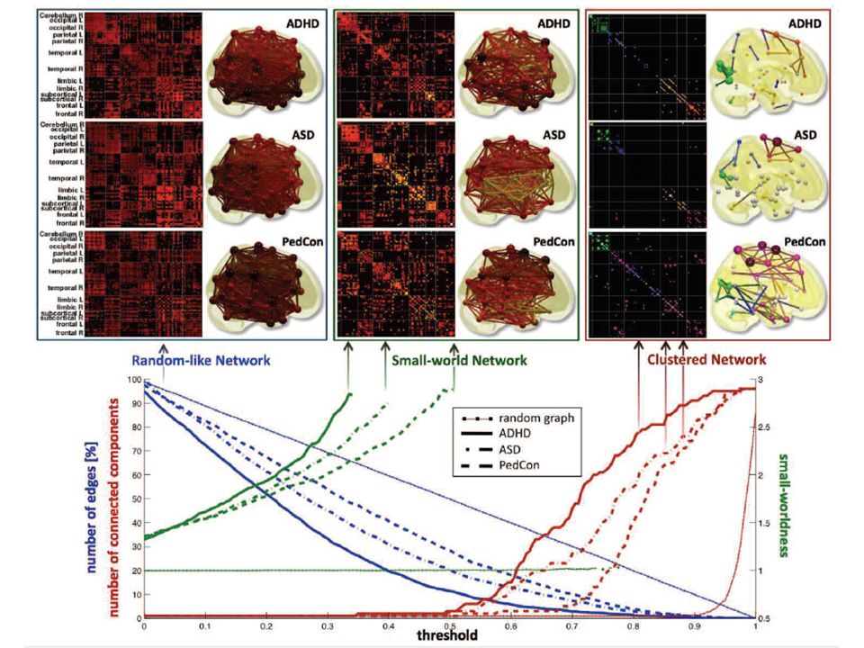
27. Discriminative persistent homology of brain networks, 2011 Hyekyoung Lee Chung, M.K.; Hyejin Kang; Bung-Nyun Kim;Dong Soo Lee
Constructing functional brain networks with 97 regions of interest (ROIs) extracted from FDG-PET data for
24 attention-deficit hyperactivity disorder (ADHD),
26 autism spectrum disorder (ASD) and
11 pediatric control (PedCon).
Data = measurement fj
taken at region j
Graph: 97 vertices representing 97 regions of interest
edge exists between two vertices i,j if correlation
between fj and fj ≥ threshold
How to choose the threshold? Don’t, instead use persistent homology

29. measurement at location i
Vertices = Regions of Interest
Create Rips complex by growing epsilon balls (i.e. decreasing threshold) where distance between two vertices is given by
where fi =
measurement at location i

30. Discriminative persistent homology of brain networks, 2011 Hyekyoung Lee Chung, M.K.; Hyejin Kang; Bung-Nyun Kim;Dong Soo Lee
Constructing functional brain networks with 97 regions of interest (ROIs) extracted from FDG-PET data for
24 attention-deficit hyperactivity disorder (ADHD),
26 autism spectrum disorder (ASD) and
11 pediatric control (PedCon).
Data = measurement fj
taken at region j
Graph: 97 vertices representing 97 regions of interest
edge exists between two vertices i,j if correlation
between fj and fj ≥ threshold
How to choose the threshold? Don’t, instead use persistent homology

32. Application to Natural Image Statistics
With V. de Silva, T. Ishkanov, A. Zomorodian

33. An image taken by black and white digital camera can be viewed as a vector, with one coordinate for each pixel
Each pixel has a “gray scale” value, can be thought of as a real number (in reality, takes one of 255 values)
Typical camera uses tens of thousands of pixels, so images lie in a very high dimensional space, call it pixel space, P

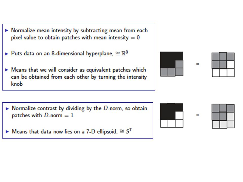
34. Lee-Mumford-Pedersen [LMP] study only high contrast patches.
Collection: 4.5 x 106 high contrast patches from a
collection of images obtained by van Hateren and van der Schaaf

39. Eurographics Symposium on Point-Based Graphics (2004)
Topological estimation using witness complexes
Vin de Silva and Gunnar Carlsson

40. Eurographics Symposium on Point-Based Graphics (2004)
Topological estimation using witness complexes
Vin de Silva and Gunnar Carlsson