1. 4.3 Diagnostic Checks VO 107.425 - Verallgemeinerte lineare Regressionsmodelle

2. Diagnostic Checks  Goodness-of-fit tests provide only global measures of the fit of a model.  Regression diagnostics aims at identifying reasons for a bad fit.  Diagnostic measures should in particular identify observations  that are not well explained by the model.  that are influential for some aspect of it.

3. 4.3.1 Residuals Residuals measure the agreement between single observations and their fitted values and help to identify poorly fitting observations that may have a strong impact on the overall fit of the model. For scaled binomial data the Pearson residual has the form: with as the estimated standard deviation as the probability for the fitted model as the number of observations

4. 4.3.1 Residuals For small n i the distribution of r p (y i, π i ) is rather skewed, an effect that is ameliorated by using the transformation to Anscombe residuals: where Ansombe residuals consider an approximation to by the use of the delta method, which yields The Pearson residuals cannot be expected to have unit variance because the variance of the residual has not been taken into account. The standardization just uses the estimated standard deviation of

5. 4.3.1 Residuals

7. residuals against ordered fitted values  if one suspects that particular values should be transformed before being included in the linear predictor residuals against corresponding quantiles of a normal distribution  Compares the standardized residuals to the order of an N(0,1)-sample. If the model is correct and residuals can be expected to be approximately normally distributed, the plot should show approximately a straight line as long as outliers are absent.

8. Example 4.3: Unemployment In a study on the duration of unemployment with sample size n = 982 we distinguish between short term unemployment ( ≤ 6 months) and long-term unemployment (> 6 months). It is shown that that for older unemployed persons the, the fitted values tend to be larger than the observed.

9. Example 4.4: Food-Stamp Data The food-stamp data from Künsch et al. (1989) consists of n = 150 persons, 24 of whom participated in the federal food-stamp program. The response indicates participation. The predictor variables represent the binary variables tenancy (TEN) supplemental income (SUP) log-transformation of monthly income log(monthly income + 1) (LMI)

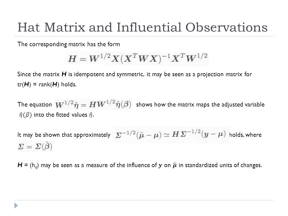
10. Hat Matrix and Influential Observations

13. 4.3.3 Case Deletion

14. Example 4.5: Unemployment Cook‘s distances for unemployment data show that observations 33, 38, 44, which correspond to ages 48, 53, 59, are influential. All three observations are rather far from the fit.

15. Example 4.6: Exposure to Dust (Non-Smokers) Observed covariates:  mean dust concentration at working place in mg/m³ (dust)  duration of exposure in years (years)  smoking (1: yes; 0: no) Binary response:  Bronchitis (1: present; 0: not present) Sample number:  n = 1246

16. Table 4.4 shows the estimated coefficient for the main effects model. Table 4.5 shows the fit without the observation (15.04, 27)  It can be seen that the coefficient for the concentration of dust has distinctly changed. Example 4.6: Exposure to Dust (Non-Smokers)

17. As seen in Figure 4.7, large values of Cook’s distance are the following observations with their respective values: 730 (1.63, 8); 1175 (8, 32); 1210 (8, 13)(dust, years) All three observations correspond to persons with bronchitis. They are NOT extreme in the range of years, which is the influential variable. The variable dust shows no significant effect, and therefore it is only a consequence that the Cool’s distance is small. Example 4.6: Exposure to Dust (Non-Smokers)

18. In this example the exposure data, including non-smokers, is used. The full dataset  concentration of dust  years of exposure  smoking are significantly influential!  one observation positioned very extreme in the observation space! Example 4.7: Exposure to Dust

19. By excluding the extreme value  coefficient estimates for the variables years and smoking are similar to the estimates for the full data set.  coefficients for the variable concentration of dust differ by about 8%. Since observation 1246 is far away from the data and the mean exposure is a variable not easy to measure  should be considered as an outlier and omitted.

20. Thank you for your attention!