1. Patterns of Decadal Climate Variability and their Impact on Rainfall and the Biosphere Peter G. Baines Dept of Civil and Environmental Engineering, University of Melbourne Australia

2. The principal patterns of variation of the observed climate over the past 100+ years, and the dynamics behind them, are coming into focus. Here I will describe these patterns, and then say something about how they affect rainfall, and also some connections between rainfall and the biosphere.

3. Of all the variables that one may use to describe climate, the most important is (probably) Sea Surface Temperature (SST), because: 1.It gives a measure of heat storage in the ocean. 2.It has a controlling effect on surface winds and pressure, over the ocean. 3.It has a controlling effect on surface humidity. The collection and interpretation of observations over the past 200 years or so now enable the estimation of global observations back to about 1850. This has mainly been done by two separate groups: the Hadley Centre at the UKMO, and Smith, Reynolds & c at NOAA /US, with ongoing upgrades.

4. There are many differences between these two data sets. These differences mainly arise from the manner in which the observations are interpolated into regions where there are none. References: HadISST1 (Rayner et al. 2003 ) erSSTv3 (Smith et al. 2008) Here, I have used data from each set from 1900 to 2009, taking annual means over years that begin in June and end the following May. These are termed ENSO-years, or E-years for short. Five-year running means have then been taken over these E-years. This covers time scales longer than ENSO. An EOF analysis is then performed on the resulting data. This gives a breakdown into patterns that may be associated with recognisable physical processes.

5. This procedure is most effective if the values of S(k,k) for k = 1,2,3.. decrease rapidly, so that most of the rest of them are small. We then have a succinct description of the data. EOFs are mathematical artifices that are effectively efficient descriptions of the data, and any particular one may or may not be a dynamical entity by itself. Via the Singular Value Decomposition Theorem (SVD), a data matrix R ij to be expressed in the form assuming m > n where the SUV denote Empirical Orthogonal Functions (EOFs), S(k,k) 2 denotes the variance of the k th EOF, andU and V are orthogonal matrices. Spatial pattern Time series

6. Mean Sea Surface Temperature, Hadley Centre HadISST1 data Data are: 5-year running means of HadISST1 and Smith- Reynolds erSSTv3, from June1900-May 2009. 5-year running means cover variance on time scales longer than ENSO

7. Comparisons – 70N-70S Left – HadISST Right – erSST EOF1 The Global Warming Pattern Variance 51.5 & 57.5%

8. Properties of the Global Warming Pattern: 1. Contains the secular trend in the data, similar to global mean temperature (IPCC) 2. Contains more than half the total variance in the data 3. The spatial pattern is approximately uniform, and mainly due to radiative processes, influenced by increasing greenhouse gases and aerosols. 4. There are some small exceptions to this uniform heating: The region near Antarctica, implying little change there A small region in the northern North Atlantic, which has cooled. - the latter may be attributed to a small slowing in the Atlantic conveyor (according to numerical model studies). 5. Wet regions get wetter, dry regions get dryer (Held & Soden2006)

9. Comparisons – 70N-70S Left – HadISST Right – erSST EOF2 The Pacific Decadal Oscillation PDO/IPO Pattern Variance: 14 & 11%

10. Comparisons – 70N-70S Left – HadISST Right – erSST EOF3 Atlantic Meridional Oscillation AMO Pattern Variance: 7.5 & 6.8%

11. Comparisons – 70N-70S Left – HadISST Right – erSST EOF4 The Pacific Gyre Oscillation PGO Pattern Variance: 5.1 & 4% These first four EOFs contain ~ 80% of variance for each data set.

12. The above describes 54.8% and 51.3% of the variance of the remainder of each of these two data sets after EOF1 has been removed. However, we may do better with complex EOFs. This involves taking the Hilbert transform of the time series T(r,t) at each spatial grid point of the data, and regarding this as the imaginary part of the time series, giving the complex time series at each position r : T(r,t) + i H(T(r,t)) One then takes the SVD of this complex matrix to obtain the complex CEOFs, again taking the real part of the results for real values. where Uc and Vc are now complex. The following calculations are for HadISST1

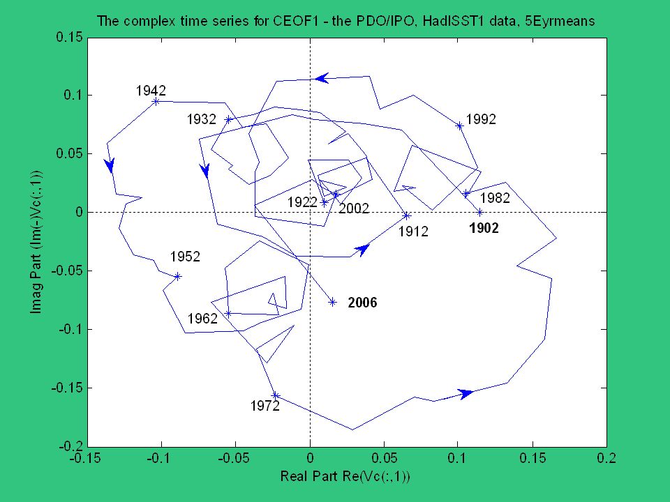
13. Complex EOF1 of HadISST1(-EOF1), 5Eyrmeans, 1900-2009 (2 nd EOF overall) The PDO/IPO 36.7% of total variance The total EOF is: realV(:,1).CEOF1re + imag(V:,1).CEOF1im

14. The Complex CEOF1 Cycle (was EOF2)

16. Properties of the PDO/IPO: 1. The cycle is focussed on the eastern equatorial Pacific, with northern and southern mid- latitudes in anti-phase. 2. Possibly forced by (relatively) high frequency ENSO events 3. Responsible for low-frequency changes in the equatorial Pacific and associated ENSO characteristics 4. A major regime shift occurred in the mid-1970s (Zhang&c1997) Despite a lot of attention, still not well understood

17. Complex EOF2 of HadISST1(-EOF1), 5Eyrmeans, 1900-2009 (3 rd EOF overall) The AMO 17.7% of total variance The total EOF is: realV(:,2).CEOF2re + imag(V:,2).CEOF2im

18. Properties of the AMO: 1. - associated with the Atlantic conveyor 2. SST signature is the Hemispheric pattern, with the largest signal in the northern North Atlantic 3. Modelling studies (HadCM3) show an inbuilt oscillation with decadal time scales. 4. A major regime shift occurred in the late 1960s (Baines & Folland 2005).

19. Complex EOF3 of HadISST1(-EOF1), 5Eyrmeans, 1900-2009 (4 th EOF overall) The PGO 11.5% of total variance CEOFs 1,2+3 contain 66% of variance The total EOF is: realV(:,3).CEOF3re + imag(V:,3).CEOF3im

21. Properties of the PGO: 1. The focus is on mid-latitudes in the North and South Pacific 2. It involves variations in the strength of the oceanic gyre, with apparently regular periodicity of ~ 35 years. 3. The mechanism for oscillations as identified by models (Latif & Barnett (1994/6)) involves thermal forcing of the atmosphere with subsequent slow evolution of the ocean.

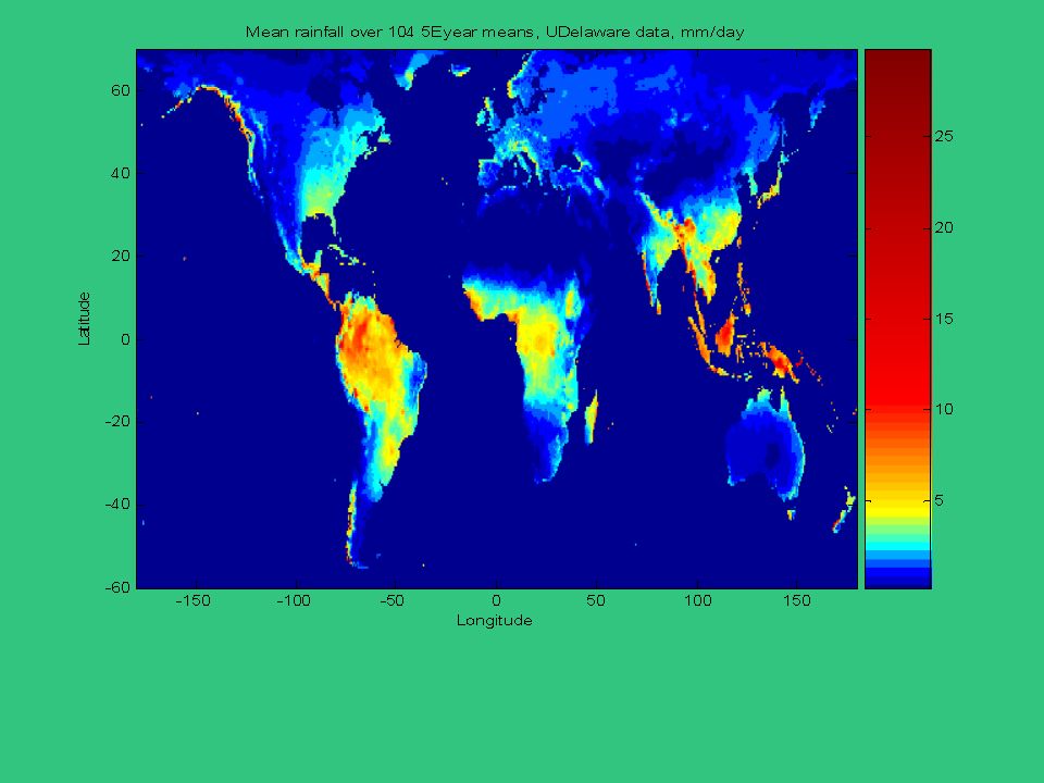
22. Rainfall

24. Projection of EOF1 of HadISST1 on Udelaware rainfall

25. Biology - fAPAR

26. Annual Mean

27. EOF1 fAPAR 68.6% of total variance

28. Mean Value of TRMM Rainfall Units: mm/hour 1998-2008 Mean value of fAPAR, 1998-2005 fAPAR is the fraction of Absorbed Photosynthetically Active Radiation, a measure of plant growth (Ref.: Gobron et al. 2006, J.Geophys. Res. 111, D13110)

29. TRMM RainfallfAPAR EOF1 of the Annual cycle of TRMM Rainfall and fAPAR Each describes 75% of the total variance of the annual cycle

30. 10 years of Sahel TRMM rainfall and fAPAR 10 years of Central African TRMM rainfall and fAPAR Annual mean rainfall

31. CONCLUSIONS 1.Four patterns (GW, PDO, AMO, PGO) dominate the variability of global climate on the decadal time scale, and of Africa in particular. The PDO, AMO and PGO are oscillatory in nature, with very different dynamics and implications for rainfall and climate variability. 2.Despite the expectations that wet regions get wetter and dry regions drier from Global Warming, data over land show increased precipitation in many areas. 3.The annual cycle of plant growth (as measured by fAPAR) follows rainfall (by ~1 month), and is much less variable (in Sahel and central Africa).

32. EOF1 EOF2 EOFs 1 (75%) and EOF2 (13.1%) of the Annual Cycle of TRMM rainfall for Africa Percentages denote fractions of variance of the annual cycle Note that EOF1 is dominant