Download presentation
Presentation is loading. Please wait.

2
Lumped Parameter Modelling UoL MSc Remote Sensing Dr Lewis plewis@geog.ucl.ac.uk

3
Introduction introduce simple lumped parameter models Build on RT modelling RT: formulate for biophysical parameters –LAI, leaf number density, size etc –investigate eg sensitivity of a signal to canopy properties e.g. effects of soil moisture on VV polarised backscatter or Landsat TM waveband reflectance –Inversion? Non-linear, many parameters

4
Linear Models For some set of independent variables x = {x 0, x 1, x 2, …, x n } have a model of a dependent variable y which can be expressed as a linear combination of the independent variables.

5
Linear Models?

6
Linear Mixture Modelling Spectral mixture modelling: –Proportionate mixture of (n) end-member spectra –First-order model: no interactions between components
 end-member spectra –First-order model: no interactions between components")
7
Linear Mixture Modelling r = {r, r, … r m, 1.0} –Measured reflectance spectrum (m wavelengths) nx(m+1) matrix:
 nx(m+1) matrix:")
8
Linear Mixture Modelling n=(m+1) – square matrix Eg n=2 (wavebands), m=2 (end-members)
 – square matrix Eg n=2 (wavebands), m=2 (end-members)")
9
Reflectance Band 1 Reflectance Band 2 1 2 3 r

10
Linear Mixture Modelling as described, is not robust to error in measurement or end-member spectra; Proportions must be constrained to lie in the interval (0,1) –- effectively a convex hull constraint; m+1 end-member spectra can be considered; needs prior definition of end-member spectra; cannot directly take into account any variation in component reflectances –e.g. due to topographic effects

11
Linear Mixture Modelling in the presence of Noise Define residual vector minimise the sum of the squares of the error e, i.e. Method of Least Squares (MLS)
.")
12
Error Minimisation Set (partial) derivatives to zero
 derivatives to zero")
13
Error Minimisation Can write as: Solve for P by matrix inversion

14
e.g. Linear Regression

15
RMSE

16
y x xx1x1 x2x2

17
Weight of Determination (1/w) Calculate uncertainty at y(x)
 Calculate uncertainty at y(x)")
18
Lumped Canopy Models Motivation –Describe reflectance/scattering but dont need biophysical parameters Or dont have enough information –Examples Albedo Angular normalisation – eg of VIs Detecting change in the signal Require generalised measure e.g cover When can calibrate model –Need sufficient ground measures (or model) and to know conditions
 and to know conditions")
19
Model Types Empirical models –E.g. polynomials –E.g. describe BRDF by polynomial –Need to guess functional form –OK for interpolation Semi-empirical models –Based on physical principles, with empirical linkages –Right sort of functional form –Better behaviour in integration/extrapolation (?)
.")
20
Linear Kernel-driven Modelling of Canopy Reflectance Semi-empirical models to deal with BRDF effects –Originally due to Roujean et al (1992) –Also Wanner et al (1995) –Practical use in MODIS products BRDF effects from wide FOV sensors –MODIS, AVHRR, VEGETATION, MERIS
 –Also Wanner et al (1995) –Practical use in MODIS products BRDF effects from wide FOV sensors –MODIS, AVHRR, VEGETATION, MERIS")
21
Satellite, Day 1 Satellite, Day 2 X

22
AVHRR NDVI over Hapex-Sahel, 1992

23
Linear BRDF Model of form: Model parameters: Isotropic Volumetric Geometric-Optics

24
Linear BRDF Model of form: Model Kernels: Volumetric Geometric-Optics

25
Volumetric Scattering Develop from RT theory –Spherical LAD –Lambertian soil –Leaf reflectance = transmittance –First order scattering Multiple scattering assumed isotropic

26
Volumetric Scattering If LAI small:

27
Volumetric Scattering Write as: RossThin kernel Similar approach for RossThick

28
Geometric Optics Consider shadowing/protrusion from spheroid on stick (Li-Strahler 1985)
")
29
Geometric Optics Assume ground and crown brightness equal Fix shape parameters Linearised model –LiSparse –LiDense

30
Kernels Retro reflection (hot spot) Volumetric (RossThick) and Geometric (LiSparse) kernels for viewing angle of 45 degrees
 Volumetric (RossThick) and Geometric (LiSparse) kernels for viewing angle of 45 degrees")
31
Kernel Models Consider proportionate ( ) mixture of two scattering effects
 mixture of two scattering effects")
32
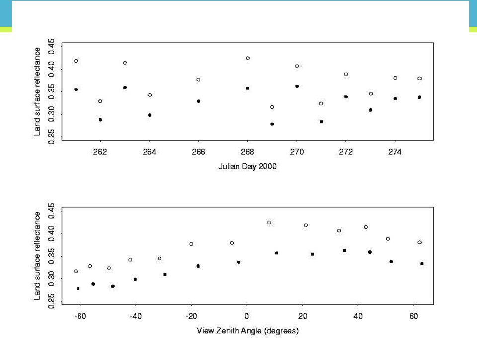
Using Linear BRDF Models for angular normalisation

35
BRDF Normalisation Fit observations to model Output predicted reflectance at standardised angles –E.g. nadir reflectance, nadir illumination Typically not stable –E.g. nadir reflectance, SZA at local mean And uncertainty via

36
Linear BRDF Models for albedo Directional-hemispherical reflectance –can be phrased as an integral of BRF for a given illumination angle over all illumination angles. –measure of total reflectance due to a directional illumination source (e.g. the Sun) –sometimes called black sky albedo. –Radiation absorbed by the surface is simply 1-
 –sometimes called black sky albedo. –Radiation absorbed by the surface is simply 1-.")
37
Linear BRDF Models for albedo

38
Similarly, the bi-hemispherical reflectance –measure of total reflectance over all angles due to an isotropic (diffuse) illumination source (e.g. the sky). –sometimes known as white sky albedo
. –sometimes known as white sky albedo.")
39
Spectral Albedo Total (direct + diffuse) reflectance –Weighted by proportion of diffuse illumination Pre-calculate integrals – rapid calculation of albedo
 reflectance –Weighted by proportion of diffuse illumination Pre-calculate integrals – rapid calculation of albedo")
40
Linear BRDF Models to track change E.g. Burn scar detection Active fire detection (e.g. MODIS) –Thermal –Relies on seeing active fire –Miss many –Look for evidence of burn (scar)
 –Thermal –Relies on seeing active fire –Miss many –Look for evidence of burn (scar).")
41
Linear BRDF Models to track change Examine change due to burn (MODIS)
")
42
MODIS Channel 5 Observation DOY 275

43
MODIS Channel 5 Observation DOY 277

44
Detect Change Need to model BRDF effects Define measure of dis-association

45
MODIS Channel 5 Prediction DOY 277

46
MODIS Channel 5 Discrepency DOY 277

47
MODIS Channel 5 Observation DOY 275

48
MODIS Channel 5 Prediction DOY 277

49
MODIS Channel 5 Observation DOY 277

50
Single Pixel

51
Detect Change Burns are: –negative change in Channel 5 –Of long (week) duration Other changes picked up –E.g. clouds, cloud shadow –Shorter duration –or positive change (in all channels) –or negative change in all channels
 –or negative change in all channels.")
52
Day of burn

53
Other Lumped Parameter Optical Models Modified RPV (MRPV) model –Multiplicative terms describing BRDF shape –Linearise by taking log
 model –Multiplicative terms describing BRDF shape –Linearise by taking log")
54
Other Lumped Parameter Optical Models Gilabert et al. –Linear mixture model Soil and canopy: f = exp(-CL) Parametric model of multiple scattering
 Parametric model of multiple scattering.")
55
Conclusions Developed semi-empirical models –Many linear (linear inversion) –Or simple form Lumped parameters –Information on gross parameter coupling –Few parameters to invert
 –Or simple form Lumped parameters –Information on gross parameter coupling –Few parameters to invert")
56
Conclusions Uses of models –E.g. linear, kernel driven –When dont need full biophysical parameterisation Forms of models –Similar forms (from RT theory) Applications: –BRDF normalisation –Albedo –Change detection
 Applications: –BRDF normalisation –Albedo –Change detection.")
Similar presentations


 Disney UCL Geography Office: 301, 3rd Floor, Chandler House Tel: 7670 4290 (x24290) Email:>")


