Download presentation
Presentation is loading. Please wait.

1
Random Regressors and Moment Based Estimation Prepared by Vera Tabakova, East Carolina University

2
10.1 Linear Regression with Random x’s 10.2 Cases in Which x and e are Correlated 10.3 Estimators Based on the Method of Moments 10.4 Specification Tests

3
The assumptions of the simple linear regression are: SR1. SR2. SR3. SR4. SR5. The variable x i is not random, and it must take at least two different values. SR6. (optional)
.")
4
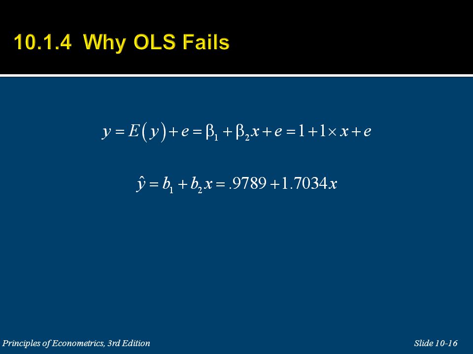
The purpose of this chapter is to discuss regression models in which x i is random and correlated with the error term e i. We will: Discuss the conditions under which having a random x is not a problem, and how to test whether our data satisfies these conditions. Present cases in which the randomness of x causes the least squares estimator to fail. Provide estimators that have good properties even when x i is random and correlated with the error e i.

5
A10.1 correctly describes the relationship between y i and x i in the population, where β 1 and β 2 are unknown (fixed) parameters and e i is an unobservable random error term. A10.2The data pairs, are obtained by random sampling. That is, the data pairs are collected from the same population, by a process in which each pair is independent of every other pair. Such data are said to be independent and identically distributed.

6
A10.3 The expected value of the error term e i, conditional on the value of x i, is zero. This assumption implies that we have (i) omitted no important variables, (ii) used the correct functional form, and (iii) there exist no factors that cause the error term e i to be correlated with x i. If, then we can show that it is also true that x i and e i are uncorrelated, and that. Conversely, if x i and e i are correlated, then and we can show that.
 omitted no important variables, (ii) used the correct functional form, and (iii) there exist no factors that cause the error term e i to be correlated with x i. If, then we can show that it is also true that x i and e i are uncorrelated, and that. Conversely, if x i and e i are correlated, then and we can show that..")
7
A10.4In the sample, x i must take at least two different values. A10.5 The variance of the error term, conditional on x i is a constant σ 2. A10.6 The distribution of the error term, conditional on x i, is normal.

8
Under assumptions A10.1-A10.4 the least squares estimator is unbiased. Under assumptions A10.1-A10.5 the least squares estimator is the best linear unbiased estimator of the regression parameters, conditional on the x’s, and the usual estimator of σ 2 is unbiased.

9
Under assumptions A10.1-A10.6 the distributions of the least squares estimators, conditional upon the x’s, are normal, and their variances are estimated in the usual way. Consequently the usual interval estimation and hypothesis testing procedures are valid.

10
Figure 10.1 An illustration of consistency

11
Remark: Consistency is a “large sample” or “asymptotic” property. We have stated another large sample property of the least squares estimators in Chapter 2.6. We found that even when the random errors in a regression model are not normally distributed, the least squares estimators still have approximate normal distributions if the sample size N is large enough. How large must the sample size be for these large sample properties to be valid approximations of reality? In a simple regression 50 observations might be enough. In multiple regression models the number might be much higher, depending on the quality of the data.

12
A10.3*

13
Under assumption A10.3* the least squares estimators are consistent. That is, they converge to the true parameter values as N . Under assumptions A10.1, A10.2, A10.3*, A10.4 and A10.5, the least squares estimators have approximate normal distributions in large samples, whether the errors are normally distributed or not. Furthermore our usual interval estimators and test statistics are valid, if the sample is large.

14
If assumption A10.3* is not true, and in particular if so that x i and e i are correlated, then the least squares estimators are inconsistent. They do not converge to the true parameter values even in very large samples. Furthermore, none of our usual hypothesis testing or interval estimation procedures are valid.

15
Figure 10.2 Plot of correlated x and e

17
Figure 10.3 Plot of data, true and fitted regressions

18
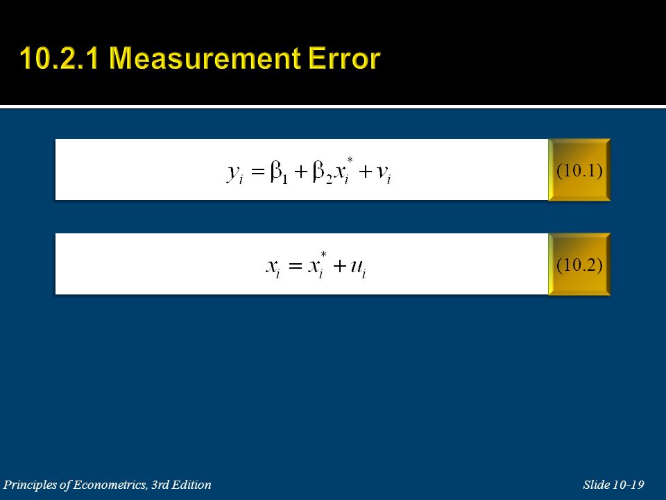
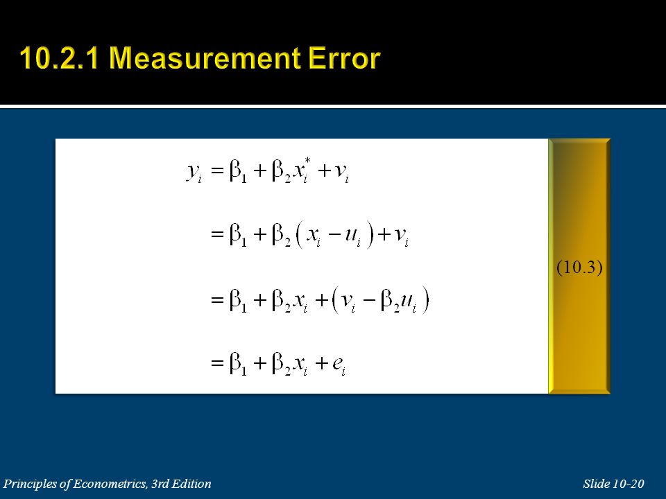
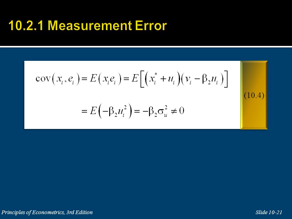
When an explanatory variable and the error term are correlated the explanatory variable is said to be endogenous and means “determined within the system.” When an explanatory variable is correlated with the regression error one is said to have an “endogeneity problem.”

22
Omitted factors: experience, ability and motivation. Therefore, we expect that

23
There is a feedback relationship between P i and Q i. Because of this feedback, which results because price and quantity are jointly, or simultaneously, determined, we can show that The resulting bias (and inconsistency) is called the simultaneous equations bias.
 is called the simultaneous equations bias..")
24
In this case the least squares estimator applied to the lagged dependent variable model will be biased and inconsistent.

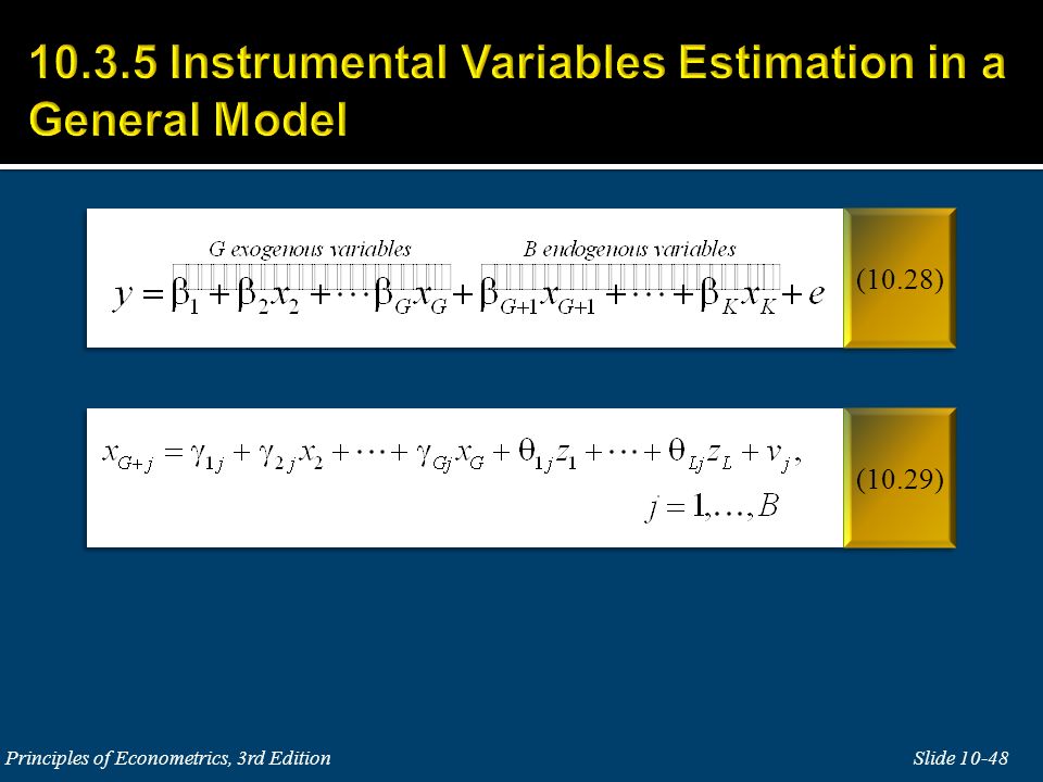
25
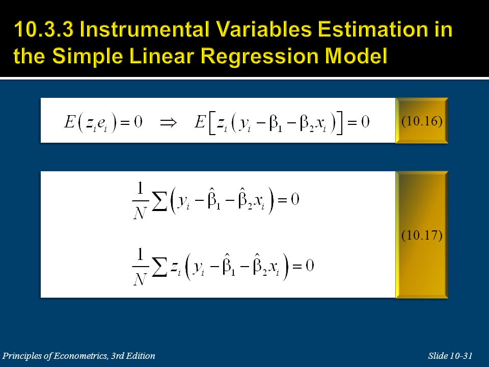
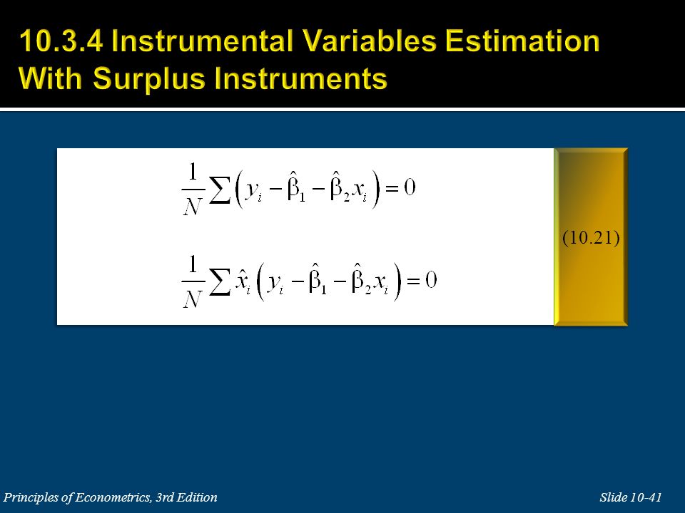
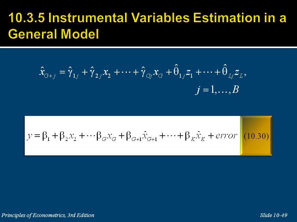
When all the usual assumptions of the linear model hold, the method of moments leads us to the least squares estimator. If x is random and correlated with the error term, the method of moments leads us to an alternative, called instrumental variables estimation, or two-stage least squares estimation, that will work in large samples.

29
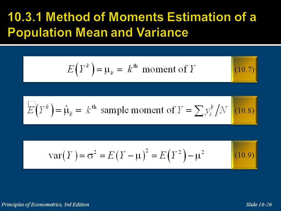
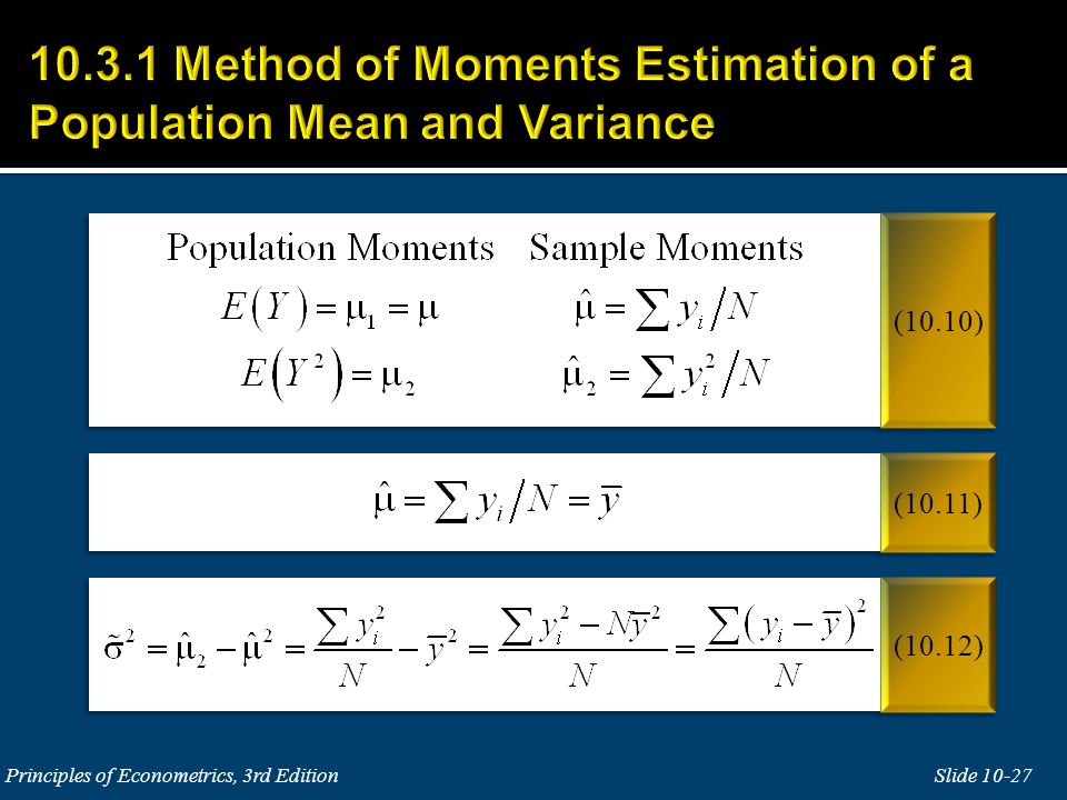
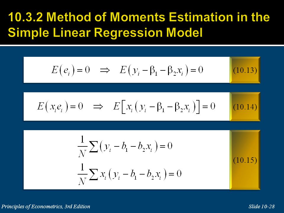
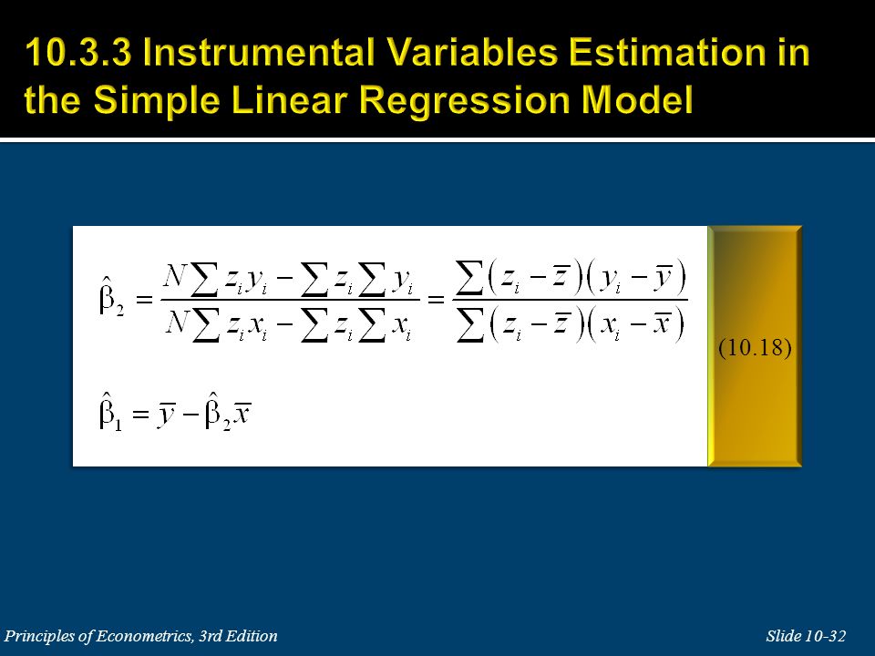
Under "nice" assumptions, the method of moments principle of estimation leads us to the same estimators for the simple linear regression model as the least squares principle.

30
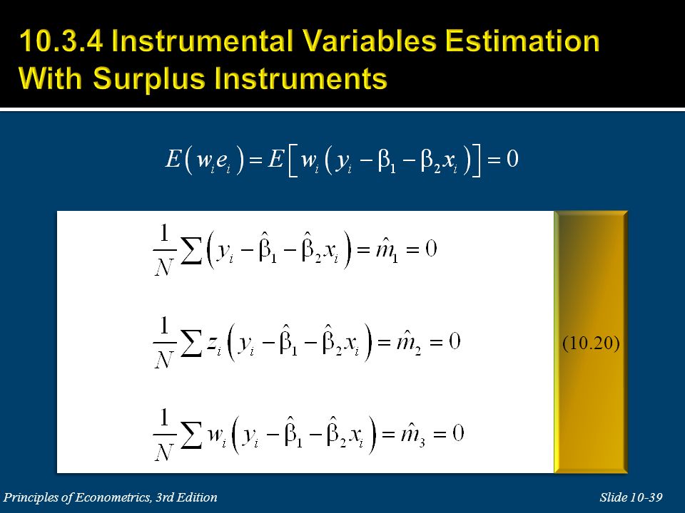
Suppose that there is another variable, z, such that z does not have a direct effect on y, and thus it does not belong on the right-hand side of the model as an explanatory variable. z i is not correlated with the regression error term e i. Variables with this property are said to be exogenous. z is strongly [or at least not weakly] correlated with x, the endogenous explanatory variable. A variable z with these properties is called an instrumental variable.

33
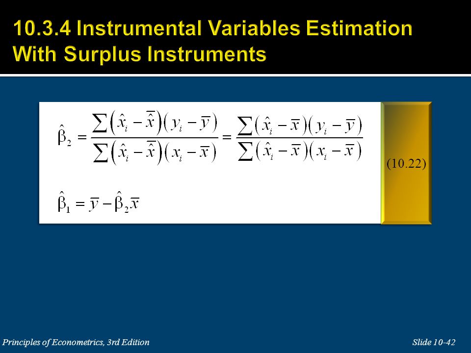
These new estimators have the following properties: They are consistent, if In large samples the instrumental variable estimators have approximate normal distributions. In the simple regression model

34
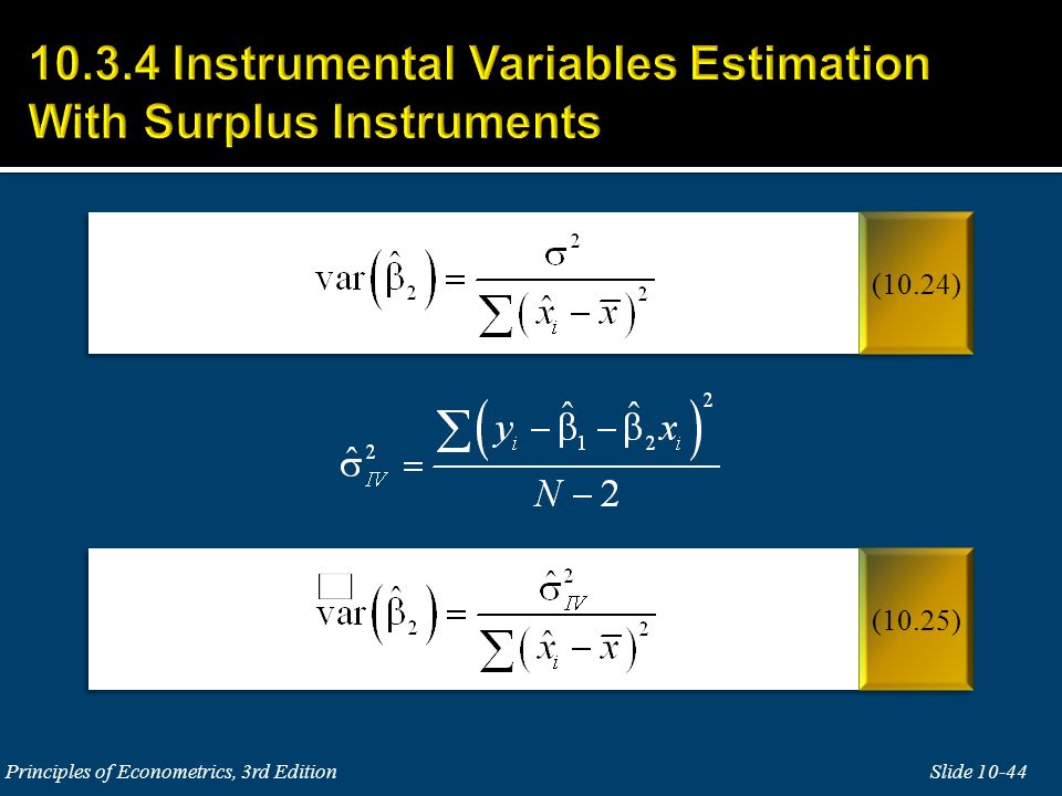
The error variance is estimated using the estimator

35
Using the instrumental variables estimation procedure when it is not required leads to wider confidence intervals, and less precise inference, than if least squares estimation is used. The bottom line is that when instruments are weak instrumental variables estimation is not reliable.

40
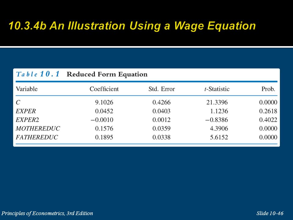
A 2-step process. Regress x on a constant term, z and w, and obtain the predicted values Use as an instrumental variable for x.

43
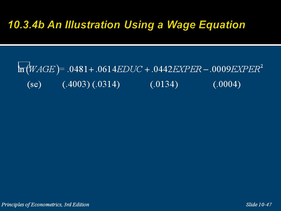
Two-stage least squares (2SLS) estimator: Stage 1 is the regression of x on a constant term, z and w, to obtain the predicted values. This first stage is called the reduced form model estimation. Stage 2 is ordinary least squares estimation of the simple linear regression

50
When testing the null hypothesis use of the test statistic is valid in large samples. It is common, but not universal, practice to use critical values, and p-values, based on the distribution rather than the more strictly appropriate N(0,1) distribution. The reason is that tests based on the t-distribution tend to work better in samples of data that are not large.
 distribution. The reason is that tests based on the t-distribution tend to work better in samples of data that are not large..")
51
When testing a joint hypothesis, such as, the test may be based on the chi-square distribution with the number of degrees of freedom equal to the number of hypotheses (J) being tested. The test itself may be called a “Wald” test, or a likelihood ratio (LR) test, or a Lagrange multiplier (LM) test. These testing procedures are all asymptotically equivalent.
 test, or a Lagrange multiplier (LM) test. These testing procedures are all asymptotically equivalent..")
52
Unfortunately R 2 can be negative when based on IV estimates. Therefore the use of measures like R 2 outside the context of the least squares estimation should be avoided.

53
Can we test for whether x is correlated with the error term? This might give us a guide of when to use least squares and when to use IV estimators. Can we test whether our instrument is sufficiently strong to avoid the problems associated with “weak” instruments? Can we test if our instrument is valid, and uncorrelated with the regression error, as required?

54
If the null hypothesis is true, both the least squares estimator and the instrumental variables estimator are consistent. Naturally if the null hypothesis is true, use the more efficient estimator, which is the least squares estimator. If the null hypothesis is false, the least squares estimator is not consistent, and the instrumental variables estimator is consistent. If the null hypothesis is not true, use the instrumental variables estimator, which is consistent.

55
Let z 1 and z 2 be instrumental variables for x. 1. Estimate the model by least squares, and obtain the residuals. If there are more than one explanatory variables that are being tested for endogeneity, repeat this estimation for each one, using all available instrumental variables in each regression.

56
2. Include the residuals computed in step 1 as an explanatory variable in the original regression, Estimate this "artificial regression" by least squares, and employ the usual t-test for the hypothesis of significance

57
3. If more than one variable is being tested for endogeneity, the test will be an F-test of joint significance of the coefficients on the included residuals.

58
If we have L > 1 instruments available then the reduced form equation is

59
1. Compute the IV estimates using all available instruments, including the G variables x 1 =1, x 2, …, x G that are presumed to be exogenous, and the L instruments z 1, …, z L. 2. Obtain the residuals

60
3. Regress on all the available instruments described in step 1. 4. Compute NR 2 from this regression, where N is the sample size and R 2 is the usual goodness-of-fit measure. 5. If all of the surplus moment conditions are valid, then If the value of the test statistic exceeds the 100(1−α)-percentile from the distribution, then we conclude that at least one of the surplus moment conditions restrictions is not valid.
-percentile from the distribution, then we conclude that at least one of the surplus moment conditions restrictions is not valid..")
61
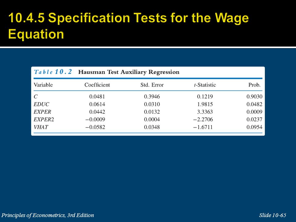
10.4.4a The Hausman Test

62
10.4.4b Test for Weak Instruments

63
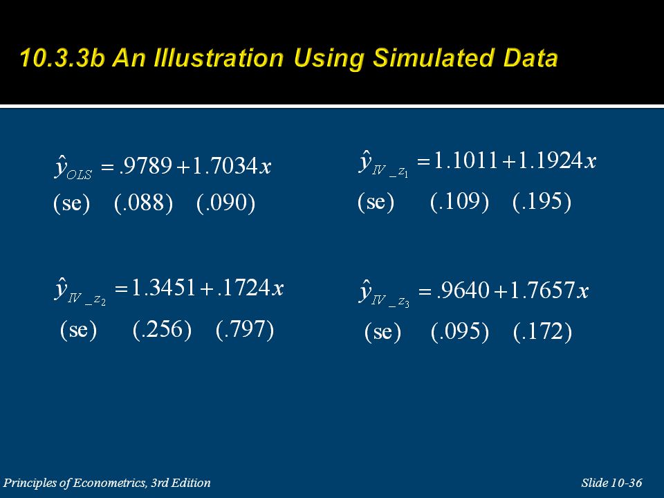
10.4.4c Testing Surplus Moment Conditions If we use z 1 and z 2 as instruments there is one surplus moment condition. The R 2 from this regression is.03628, and NR 2 = 3.628. The.05 critical value for the chi-square distribution with one degree of freedom is 3.84, thus we fail to reject the validity of the surplus moment condition.

64
10.4.4c Testing Surplus Moment Conditions If we use z 1, z 2 and z 3 as instruments there are two surplus moment conditions. The R 2 from this regression is.1311, and NR 2 = 13.11. The.05 critical value for the chi-square distribution with two degrees of freedom is 5.99, thus we reject the validity of the two surplus moment conditions.

66
Slide 10-66Principles of Econometrics, 3rd Edition asymptotic properties conditional expectation endogenous variables errors-in-variables exogenous variables finite sample properties Hausman test instrumental variable instrumental variable estimator just identified equations large sample properties over identified equations population moments random sampling reduced form equation sample moments simultaneous equations bias test of surplus moment conditions two-stage least squares estimation weak instruments

67
Slide 10-67Principles of Econometrics, 3rd Edition

68
10A.1 Conditional Expectations Principles of Econometrics, 3rd EditionSlide 10-68 (10A.1)
")
69
10A.2 Iterated Expectations Principles of Econometrics, 3rd EditionSlide 10-69 (10A.2)
")
70
10A.2 Iterated Expectations Principles of Econometrics, 3rd EditionSlide 10-70

71
10A.2 Iterated Expectations Principles of Econometrics, 3rd EditionSlide 10-71 (10A.3) (10A.4)
 (10A.4)")
72
10A.3 Regression Model Applications Principles of Econometrics, 3rd EditionSlide 10-72 (10A.5) (10A.6) (10A.7)
 (10A.6) (10A.7)")
73
Principles of Econometrics, 3rd EditionSlide 10-73

74
Principles of Econometrics, 3rd EditionSlide 10-74 (10B.1) (10B.2) (10B.3)
 (10B.2) (10B.3)")
75
Principles of Econometrics, 3rd EditionSlide 10-75 (10B.4)
")
76
Principles of Econometrics, 3rd EditionSlide 10-76 (10C.1) (10C.2)
 (10C.2)")
77
Principles of Econometrics, 3rd EditionSlide 10-77 (10C.3) (10C.4)
 (10C.4)")
78
Principles of Econometrics, 3rd EditionSlide 10-78 (10D.4) (10D.1) (10D.2) (10D.3)
 (10D.1) (10D.2) (10D.3)")
79
Principles of Econometrics, 3rd EditionSlide 10-79 (10D.8) (10D.5) (10D.6) (10D.7)
 (10D.5) (10D.6) (10D.7)")
80
Principles of Econometrics, 3rd EditionSlide 10-80 (10D.9)
")
Similar presentations


>")


