2. Recap Summary of Chapter 6 Interpolation Linear Interpolation

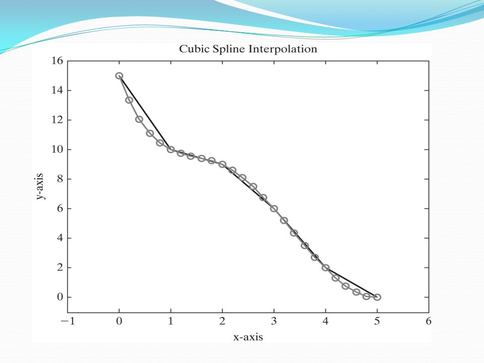
3. Cubic Spline Interpolation Connecting data points with straight lines probably isn’t the best way to estimate intermediate values, although it is surely the simplest A smoother curve can be created by using the cubic spline interpolation technique, included in the interp1 function. This approach uses a third-order polynomial to model the behavior of the data To call the cubic spline, we need to add a fourth field to interp1 : interp1(x,y,3.5,'spline') This command returns an improved estimate of y at x = 3.5: ans = 3.9417 The cubic spline technique can be used to create an array of new estimates for y for every member of an array of x -values: new_x = 0:0.2:5; new_y_spline = interp1(x,y,new_x,'spline'); A plot of these data on the same graph as the measured data using the command plot(x,y,new_x,new_y_spline,'-o') results in two different lines

6. Multidimensional Interpolation Suppose there is a set of data z that depends on two variables, x and y. For example

7. Continued…. In order to determine the value of z at y = 3 and x = 1.5, two interpolations have to performed One approach would be to find the values of z at y = 3 and all the given x -values by using interp1 and then do a second interpolation in new chart First let’s define x, y, and z in MATLAB : y = 2:2:6; x = 1:4; z = [ 7 15 22 30 54 109 164 218 403 807 1210 1614]; Now use interp1 to find the values of z at y = 3 for all the x -values: new_z = interp1(y,z,3) returns new_z = 30.50 62.00 93.00 124.00 Finally, since we have z -values at y = 3, we can use interp1 again to find z at y = 3 and x = 1.5: new_z2 = interp1(x,new_z,1.5) new_z2 = 46.25

8. Continued…. Although the previous approach works, performing the calculations in two steps is awkward MATLAB includes a two-dimensional linear interpolation function, interp2, that can solve the problem in a single step: interp2(x,y,z,1.5,3) ans = 46.2500 The first field in the interp2 function must be a vector defining the value associated with each column (in this case, x ), and the second field must be a vector defining the values associated with each row (in this case, y ) The array z must have the same number of columns as the number of elements in x and must have the same number of rows as the number of elements in y The fourth and fifth fields correspond to the values of x and of y for which you would like to determine new z -values

9. Continued…. MATLAB also includes a function, interp3, for three- dimensional interpolation Consult the help feature for the details on how to use this function and interpn, which allows you to perform n - dimensional interpolation All these functions default to the linear interpolation technique but will accept any of the other techniques

10. Curve Fitting Although interpolation techniques can be used to find values of y between measured x -values, it would be more convenient if we could model experimental data as y=f(x) Then we could just calculate any value of y we wanted If we know something about the underlying relationship between x and y, we may be able to determine an equation on the basis of those principles MATLAB has built-in curve-fitting functions that allow us to model data empirically These models are good only in the region where we’ve collected data If we don’t understand why a parameter such as y changes as it does with x, we can’t predict whether our data-fitting equation will still work outside the range where we’ve collected data

11. Linear Regression The simplest way to model a set of data is as a straight line Suppose a data set x = 0:5; y = [15, 10, 9, 6, 2, 0]; If we plot the data, we can try to draw a straight line through the data points to get a rough model of the data’s behavior This process is sometimes called “eyeballing it”— meaning that no calculations were done, but it looks like a good fit

12. Continued…. Looking at the plot, there are several of the points appear to fall exactly on the line, but others are off by varying amounts In order to compare the quality of the fit of this line to other possible estimates, we find the difference between the actual y -value and the value calculated from the estimate. This difference is called the residual

13. Continued….

15. The linear regression technique uses an approach called least squares fit to compare how well different equations model the behavior of the data In this technique, the differences between the actual and calculated values are squared and added together. This has the advantage that positive and negative deviations don’t cancel each other out MATLAB could be used to calculate this parameter for data. We have sum_of_the_squares = sum((y-y_calc).^2) which gives us sum_of_the_squares =5

16. Continued…. Linear regression is accomplished in MATLAB with the polyfit function Three fields are required by polyfit : a vector of x –values a vector of y –values an integer indicating what order polynomial should be used to fit the data Since a straight line is a first-order polynomial, enter the number 1 into the polyfit function: polyfit(x,y,1) ans = -2.9143 14.2857 The results are the coefficients corresponding to the best-fit first-order polynomial equation: y = -2.9143x + 14.2857 Calculate the sum of the squares to find out that if this is a better fit than “eyeballed” model or not: best_y = -2.9143*x+14.2857; new_sum = sum((y-best_y).^2) new_sum = 3.3714 Since the result of the sum-of-the-squares calculation is indeed less than the value found for the “eyeballed” line, we can conclude that MATLAB found a better fit to the data We can plot the data and the best-fit line determined by linear regression to try to get a visual sense of whether the line fits the data well: plot(x,y,'o',x,best_y)

18. Polynomial Regression

19. Continued…. We can find the sum of the squares to determine whether these models fit the data better: y2 = 0.0536*x.^2-3.182*x + 14.4643; sum((y2-y).^2) ans = 3.2643 y3 = -0.0648*x.^3+0.5398*x.^2-4.0701*x + 14.6587 sum((y3-y).^2) ans = 2.9921 The more terms we add to our equation, the “better” is the fit, at least in the sense that the distance between the measured and predicted data points decreases

20. Continued…. In order to plot the curves defined by these new equations, more than the six data points are used in the linear model MATLAB creates plots by connecting calculated points with straight lines, so if a smooth curve is needed, more points are required We can get more points and plot the curves with the following code: smooth_x = 0:0.2:5; smooth_y2 = 0.0536*smooth_x.^2-3.182*smooth_x + 14.4643; subplot(1,2,1) plot(x,y,'o',smooth_x,smooth_y2) smooth_y3 = -0.0648*smooth_x.^3+0.5398*smooth_x.^2-4.0701* smooth_x + 14.6587; subplot(1,2,2) plot(x,y,'o',smooth_x,smooth_y3)

22. The Polyval Function The polyfit function returns the coefficients of a polynomial that best fits the data, at least on the basis of a regression criterion In the previous section, we entered those coefficients into a MATLAB expression for the corresponding polynomial and used it to calculate new values of y The polyval function can perform the same job without having to reenter the coefficients The polyval function requires two inputs The first is a coefficient array, such as that created by polyfit The second is an array of x -values for which we would like to calculate new y –values For example: coef = polyfit(x,y,1) y_first_order_fit = polyval(coef,x) These two lines of code could be shortened to one line by nesting functions: y_first_order_fit = polyval(polyfit(x,y,1),x)

23. Continued…. So according to new understanding of the polyfit and polyval functions to write a program to calculate and plot the fourth- and fifth-order fits for the data y4 = polyval(polyfit(x,y,4),smooth_x); y5 = polyval(polyfit(x,y,5),smooth_x); subplot(1,2,1) plot(x,y,'o',smooth_x,y4) axis([0,6,-5,15]) subplot(1,2,2) plot(x,y,'o',smooth_x,y5) axis([0,6,-5,15])

25. The Interactive Fitting Tools MATLAB includes new interactive plotting tools that allow to annotate plots without using the comman window MATLAB also included Basic curve fitting More complicated curve fitting Statistical tools

26. Basic Curve Fitting To access the basic fitting tools, first create a figure: x = 0:5; y = [0,20,60,68,77,110] plot(x,y,'o') axis([-1,7,- 20,120]) These commands produce a graph with some sample data

27. Continued…. To activate the curve-fitting tools, select Tools -> Basic Fitting from the menu bar in the figure The basic fitting window opens on top of the plot By checking linear, cubic, and show equation, plot is generated

28. Continued…. Checking the plot residuals box generates a second plot, showing how far each data point is from the calculated line

29. Continued…. In the lower right-hand corner of the basic fitting window is an arrow button. Selecting that button twice opens the rest of the window

30. Continued…. The center panel of the window shows the results of the curve fit and offers the option of saving those results into the workspace The right-hand panel allows to select x -values and calculate y - values based on the equation displayed in the center panel

31. Continued…. In addition to the basic fitting window, the data statistics window can be accessed from the figure menu bar Select Tools -> Data Statistics from the figure window The data statistics window allows to calculate statistical functions such as the mean and standard deviation interactively, based on the data in the figure, and allows to save the results to the workspace

32. Curve-Fitting Toolbox In addition to the basic fitting utility, MATLAB contains toolboxes to help to perform specialized statistical and data-fitting operations In particular, the curve-fitting toolbox contains a graphical user interface (GUI) that allows to fit curves with more than just polynomials The curve-fitting toolbox must be installed in copy of MATLAB before execution the examples that follow

33. Example The data we’ve x = 0:5; y = [0,20,60,68,77,110]; To open the curve-fitting toolbox, type cftool This launches the curve- fitting tool window Now tell the curve-fitting tool what data to use Select the data button, which will open a data window The data window has access to the workspace and will let you select an independent (x) and dependent (y) variable from a drop-down list

34. Example Continued…. Choose x and y, respectively, from the drop-down lists A data-set name can be assigned, or MATLAB will assign one automatically Once chosen variables have been chosen, MATLAB plots the data At this point, the data window can be closed Going back to the curve-fitting tool window, now select the Fitting button that offers you choices of fitting algorithms Select New fit, and select a fit type from the Type of fit list Chose an interpolated scheme that forces the plot through all the points, and a third-order polynomial

36. Numerical Integration

37. Continued….

39. MATLAB includes two built-in functions, quad and quadl, which will calculate the integral of a function without requiring the user to specify how the rectangles (shown in previous slide) are defined The two functions differ in the numerical technique used Functions with singularities may be solved with one approach or the other, depending on the situation The quad function uses adaptive Simpson quadrature: quad('x.^2',0,1) ans = 0.3333 The quadl function uses adaptive Lobatto quadrature: quadl('x.^2',0,1) ans =0.3333

40. Continued….