1. Coupling of Atmospheric and Hydrologic Models: A Hydrologic Modeler’s Perspective George H. Leavesley 1, Lauren E. Hay 1, Martyn P. Clark 2, William J. Gutowski, Jr. 3, and Robert. L. Wilby 4 1 U.S. Geological Survey, Denver, CO 2 University of Colorado, Boulder, CO 3 Iowa State University, Ames, IA 4 King’s College London, London, UK

2. Topics Water resources issues Hydrologic modeling approaches Spatial and temporal distribution issues Hydrologic forecasting methodologies Downscaling approaches and applications

3. Water Resources Simulation and Forecast Needs Long-term Policy and Planning (10’s of years) Annual to Inter-annual Operational Planning (6 - 24 months) Short-term Operational Planning (1 - 30 days) Flash flood forecasting (hours) Land-use change and climate variability

4. PRMS

5. PRMS Snowpack Energy-Balance Components

6. LUMPED MODELS LUMPED MODELS - No account of spatial variability of processes, input, boundary conditions, and system geometry DISTRIBUTED MODELS DISTRIBUTED MODELS - Explicit account of spatial variability of processes, input, boundary conditions, and watershed characteristics QUASI-DISTRIBUTED MODELS QUASI-DISTRIBUTED MODELS - Attempt to account for spatial variability, but use some degree of lumping in one or more of the modeled characteristics. SPATIAL CONSIDERATIONS

7. MAXIMUM TEMPERATURE- ELEVATION RELATIONS

8. PRECIPITATION-ELEVATION RELATIONS

9. Precipitation and Temperature Distribution Methodologies Elevation adjustments Thiessan polygons Inverse distance weighting Geostatistical techniques XYZ method …

10. Monthly Multiple Linear Regression (MLR) equations developed for PRCP, TMAX, and TMIN using the predictor variables of station location (X, Y) and elevation (Z). XYZ Methodology

11. XYZ DISTRIBUTION

12. San Juan Basin Observation Stations 37 XYZ Spatial Redistribution of Precipitation & Temperature 1. Develop Multiple Linear Regression (MLR) equations (in XYZ) for PRCP, TMAX, and TMIN by month using all appropriate regional observation stations.

13. 2. Daily mean PRCP, TMAX, and TMIN computed for a subset of stations (3) determined by the Exhaustive Search analysis to be best stations 3. Daily station means from (2) used with monthly MLR xyz relations to estimate daily PRCP, TMAX, and TMIN on each HRU according to the XYZ of each HRU Precipitation and temperature stations XYZ Spatial Redistribution

14. Z PRCP 2. PRCP mru = slope*Z mru + intercept where PRCP mru is PRCP for your modeling response unit Z mru is mean elevation of your modeling response unit x One predictor (Z) example for distributing daily PRCP from a set of stations: 1.For each day solve for y-intercept intercept = PRCP sta - slope*Z sta where PRCP sta is mean station PRCP and Z sta is mean station elevation slope is monthly value from MLRs Plot mean station elevation (Z) vs. mean station PRCP Slope from monthly MLR used to find the y-intercept XYZ Methodology

15. XYZ DISTRIBUTION EXHAUSTIVE SEARCH ANALYSIS Select best station subset from all stations Estimate gauge undercatch error for snow events (Bias in observed data) Select precipitation frequency station set (Bias in observed data)

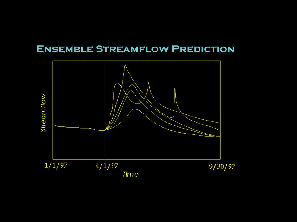
16. Forecast Methodologies - Historic data as analog for the future Ensemble Streamflow Prediction (ESP) -Synthetic time-series Weather Generator - Atmospheric model output Dynamical Downscaling Statistical Downscaling

17. Animas River @ Durango MeasuredSimulated

18. Animas Basin Snow-covered Area Year 2000 Simulated Measured (MODIS Satellite) Error Range <= 0.1

20. Probability of Exceedance ESP – Animas River @ Durango (Frequency Analysis on Peak Flows)

21. ESP – Animas River @ Durango Forecast 4/2/05 Observed 4/3 – 6/30/05

22. Representative Elevation of Atmospheric Model Output based on Regional Station Observations Elevation-based Bias Correction

23. Performance Measures Coefficient of Efficiency E Nash and Sutcliffe, 1970, J. of Hydrology Widely used in hydrology Range – infinity to +1.0 Overly sensitive to extreme values

24. Nash-Sutcliff Coefficient of Efficiency Scores Simulated vs Observed Daily Streamflow Animas River, Colorado USA

25. Statisticalvs Dynamical D Dynamical Downscaling

26. NC E P National Centers for Environmental Prediction/National Center for Atmospheric Research ReanalysisNCEP Global-scale model

27. NCEP 210 km grid spacing Retroactive 51 year record Every 5 days there is an 8-day forecast

28. Compare SDS and DDS output by using it to drive the distributed hydrologic model PRMS in 4 basins (DAY 0)

29. East Fork of the Carson Cle Elum Animas Alapaha Snowmelt Dominated 922 km 2 Snowmelt Dominated 526 km 2 Snowmelt Dominated 1792 km 2 Rainfall Dominated 3626 km 2 Study Basins

30. Statistical Downscaling Carson Cle Elum Animas Alapaha NCEP Grid nodes Basins 500km Buffer radius

31. Dynamical Downscaling 52 km grid node spacing 10 year run Regional Climate Model – RegCM2 nested within NCEP

32. Dynamical Downscaling East Fork of the Carson Cle Elum Animas Alapaha

33. Animas River Basin RegCM2 grid nodes Buffer 52 km Dynamical Downscaling Use grid-nodes that fall within 52km buffered area

34. Climate Stations 1.Station Data - BEST-STA Stations used to calibrate the hydrologic model Input Data Sets used in Hydrologic Model

35. Climate Stations 1.Station Data - BEST-STA Input Data Sets used in Hydrologic Model - ALL-STA All stations within the RegCM2 buffered area (excluding BEST-STA)

36. RegCM2 Grid Nodes 1.Station Data - BEST-STA Input Data Sets used in Hydrologic Model 2. DDS - ALL-STA

37. 1.Station Data - BEST-STA Input Data Sets used in Hydrologic Model 2. DDS 3. SDS - ALL-STA NCEP Grid Nodes

38. 1.Station Data - BEST-STA Input Data Sets used in Hydrologic Model 2. DDS 3. SDS 4. NCEP - ALL-STA

39. Nash-Sutcliffe Goodness of Fit Statistic Computed between measured and simulated runoff Best-Sta

40. Nash-Sutcliffe Goodness of Fit Statistic Computed between measured and simulated runoff Best-Sta

41. INPUT TIME SERIES: Test1 Best-Sta PRCP Bias-DDS TMAX Bias-DDS TMIN Test2 Bias-DDS PRCP Best-Sta TMAX Bias-DDS TMIN Test3 Bias-DDS PRCP Bias-DDS TMAX Best-Sta TMIN Nash-Sutcliffe Goodness of Fit Statistic Computed between measured and simulated runoff Best-Sta

42. R-Square Values between Daily “Best” timeseries and: All-Sta, Bias-All, DDS, Bias-DDS, NCEP, Bias-NCEP, and SDS Minimum Temperature Maximum Temperature Precipitation Alapaha Animas Carson Cle Elum R-Square All-Sta DDS Bias-All Bias-DDS NCEP Bias-NCEP SDS All-Sta DDS Bias-All Bias-DDS NCEP Bias-NCEP SDS All-Sta DDS Bias-All Bias-DDS NCEP Bias-NCEP SDS

43. Rainfall-dominated basin – highly controlled by daily variations in precipitation Snowmelt-dominated basins – highly controlled by daily variations in temperature and radiation Minimum Temperature Maximum Temperature Precipitation Alapaha Animas Carson Cle Elum R-Square All-Sta DDS Bias-All Bias-DDS NCEP Bias-NCEP SDS All-Sta DDS Bias-All Bias-DDS NCEP Bias-NCEP SDS All-Sta DDS Bias-All Bias-DDS NCEP Bias-NCEP SDS

44. Compare SDS and ESP Forecasts using PRMS Perfect model scenario -Ensemble Spread Range in forecasts -Ranked Probability Score measure of probabilistic forecast skill forecasts are increasingly penalized as more probability is assigned to event categories further removed from the actual outcome

45. Ranked Probability Skill Score (RPSS) for forecast days 0-8 and month using measured runoff and simulated runoff produced using: (1) SDS output and (2) ESP technique Forecast Day Month J F M A M J J A S O N D 8642086420 8642086420 0.1 0.3 0.5 0.7 0.9RPSS ESP SDS Perfect Forecast: RPSS=1

46. Forecast Spread for forecast days 0-8 and month using measured runoff and simulated runoff produced using: (1) SDS output and (2) ESP technique Forecast Day Month J F M A M J J A S O N D 8642086420 8642086420 500 1500 2500 3500 4500 Forecast Spread ESP SDS

47. Comparison of hydrologic model inputs -- Precipitation Forecast Day Month J F M A M J J A S O N D 8642086420 8642086420 0.1 0.2 0.3 0.4 0.5 Pearson Correlation ESP SDS R-square values calculated between daily basin-mean measured and (1) SDS and (2) ESP precipitation values Daily basin precipitation mean by month and forecast day for ESP (red line) and SDS (boxplot)

48. Comparison of hydrologic model inputs – Maximum Temperature Forecast Day Month J F M A M J J A S O N D 8642086420 8642086420 0.1 0.3 0.5 0.7 0.9 Pearson Correlation ESP SDS R-square values calculated between daily basin-mean measured and (1) SDS and (2) ESP maximum temperature values Daily basin maximum temperature mean by month and forecast day for ESP (red line) and SDS (boxplot)

49. Nested Domains for MM5

50. Evaluating MM5 Output Using PRMS

51. HRU Configurations

52. Daily Precipitation Mean by Month Percent Rain Days by Month XYZ vs MM5

53. Daily Basin Maximum and Minimum Temperature Mean by Month XYZ vs MM5

54. HRU Configurations

55. Results Wet period Dry period 5 Years of data 2-yr calibration 3-year evaluation

56. Improving Flash Flood Prediction Through a Synthesis of NASA Products, NWP Models and Flash Flood Decision Support Systems NASA NOAA NCAR USGS

57. Proposed Flash Flood Prediction Program Components 1km Noah LSM in the LIS framework (ensemble mode) WRF (ensemble runs) DSS – USGS Modular Modeling System (MMS) –Sacremento –CASC2D –PRMS Forecasts –15 minutes out to 24 hours –1 km resolution

58. USGS Modular Modeling System (MMS) Toolbox for Modeling, Analysis, and DSS Development and Application

59. Summary Statistical and dynamical downscaling can provide reasonable input to drive hydrologic models for a variety of applications. Statistical downscaling with XYZ distribution –handles spatial and elevation effects –most effective for frontal type storms –limited value for convective storm systems –based on historic climatology which may limit use for future climate scenarios

60. Summary Dynamical downscaled output handles spatial and elevational effects, and frontal and convective storm types. However bias correction required which results in similar limit on use with future climate scenarios. Statistical downscaling shows improvements over ESP based simulations for short-term forecasts.

61. Summary Demonstrated higher degree skill of one method over the over varies with the climatic and physiographic region of the world and the performance measures. Need for hydrologic and atmospheric modelers to work collaboratively to improve downscaling methods. Each community can provide valuable feedback to the other.