1. Environmental change and statistical trends – some examples Marian Scott Dept of Statistics, University of Glasgow NERC September 2010

2. questions about trends and change one of the most common questions common in official and policy documents- often based on simple indicators draws together much of preceeding technical sessions- time series, regression, even spatial… some challenging issues to consider

3. Observed temperature trend in Europe (EEA signals 2004). Global average temp increased by 0.7 0.2°C over the past 100 years Change in different periods of the year may have different effects, – start of the growing season determined by spring and autumn temps, – changes in winter important for species survival.

4. Climate change in Scotland (SNIFFER report, 2006) Annual average 24- hour maximum temperature over 90 year period, in 3 regions of Scotland – Very varied, non monotonic

5. Arctic ice contd Straight line tracks an 8% decline per decade Coverage is now 20% less than the 1978-2000 average

6. What is the state and trend in biodiversity (EEA CSI 009) Populations of common and widespread farmland bird species in 2003 are only 71% of their 1980 levels. Key message: Butterfly and bird species across Europe show population declines of between -2% and -37% since the early 1970s.

7. Water quality- freshwater (CSI 020) Concentrations of P generally decreased Nitrate concentrations have remained constant What are the rates of change and are they significant?

8. Bathing water quality (CSI 022) Is bathing water quality improving? In 2003, 97% of coastal bathing waters and 92% of inland bathing waters complied with the mandatory standards compared to 1993 when corresponding figures were 75% and 30%.

9. Measurement and assessment of change What it the status quo in environmental science? In time – A simple trend line – A p-value or a 95% confidence interval for the slope – A smooth curve – The relative change in an index between two time points (%) Is this sufficient?

10. Measurement and assessment of change- common tools In time (SNIFFER, 2006) – A linear regression equation was calculated for each dataset and then the trend was calculated from the gradient parameter (i.e. the rate of change) multiplied by the length of the data period to provide a clear change value since the start of the period. the significance of trends was tested using the non- parametric Mann-Kendall tau test (Sneyers, 1990). Linear trends with the Mann-Kendall significance test are widely used in the analysis of climate trends

11. Trends

12. Joint Nature Conservation Council definition of trend a trend is a measurement of change derived from a comparison of the results of two or more statistics. A trend relates to a range of dates spanning the statistics from which it is derived, e.g. 1996 - 2000. A trend will generally be expressed as a percentage change (+ for an increase, - for a decrease) or as an index.

13. Statistical definition of trend What is a statistical trend? – A long-term change in the mean level (Chatfield, 1996) – Long-term movement (Kendall and Ord, 1990) – The non-random function (t)= E (Y(t)) (Diggle, 1990) Trend is a long-term behaviour of the process, trends in mean, variance and extremes may be of interest (Chandler, this course) Environmental change often but not always means a statistical trend Not restricted to linear (or even monotonic) trends

14. Statistical tools for exploring and quantifying trend Exploratory tools – Time series plots, smoothed trends over time (are the series equally spaced, no missing data?) More formal tools – Can you assume monotonicity?, is the trend linear? – Non-parametric estimation and testing (classic tests) – Semi-parametric and non-parametric additive models (for irregular spaced data) what is monotonic? steadily increasing or decreasing

15. Visualising change

16. Time series plots Bar charts Smoothers Linear regression Space and time Pairs of images

17. two time series- what are the trends? are they monotonic? Example 1: an index of bird species population

18. two time series- what are the trends? are they monotonic? Example 1: a linear trend

19. two time series- what are the trends? are they monotonic? Example 1: a non-monotonic trend

20. Modelling the trend smoothing models (such as the moving average or LOESS curves) Y t = t + t t is underlying mean at time t, we might want to model it parametrically but t may be autocorrelated Such a model not well suited to prediction/forecasting

21. Example: The river Nile data Volume of the river for approx 100 year period. is there evidence of a change? if yes, when and in what way?

22. a non-parametric model for the Nile a smooth function (LOESS) or non- parametric regression model OK? any suggestion that there may be a change- point? (which is what?)

23. the simple problem – change in mean value here we imagine a series with two mean levels 20 observations N(10,2 2 ) and 20 observations N(20, 2 2 ) our ability to detect a change depends on the size of the change and the variability in the series

24. some simple examples

25. exploring whether a changepoint exists principle for this method concerns a comparison of a left and right smooth and difference between them confidence bands indicated, look for whether the left and right smooths leave the blue band

26. An alternative model for the Nile two smooth sections, broken at roughly 1900. different mean levels in the two periods so modelling the two periods separately

27. Parametric trend (regression) we imagine t has a known function form, e.g linear Model Y t = 0 + 1 t + t what assumptions do we make? – commonly we assume that the are uncorrelated – the regular linear model assumptions (Normality) Complications: autocorrelation, seasonality…..

28. Parametric trend Complications: autocorrelation, seasonality….. – Autocorrelation affects the standard errors of the estimates of 0 and 1 – often the magnitude of the trend is small compared to the magnitude of any seasonal component so we may need to find ways of fitting linear (and other) models where we have autocorrelated errors- which means we may also need to model the form of the autocorrelation.

29. Parametric trend (time series) identifying the autocorrelation structure is usually done by studying the ACF. Two main models- Autoregressive (AR) and Moving average (MA) to interpret the patterns in ACF we need to have a stationary series- constant mean, constant variance and the correlation between Y t and Y t+k depends on k (the lag)

30. dealing with non stationary series symptoms- obvious trends in time series plot, slowly decaying ACF from the time series session, we know that we can use several tools to create a stationary series, the most natural is differencing.

31. Time series regression account for autocorrelation using generalised least squares or by incorporating previous Y values into regression equation May lead to what are known as Box-Jenkins time series models- to find models for autocorrelated sequences (ARIMA is such a model) can be used for prediction (often called forecasting in time series literature)

32. Steps in prediction identify model (hopefully simple, so AR(1)) Fit model (includes trend and seasonality and autocorrelation) using arima() command check model (especially ACF of residuals) if OK use model for prediction – predict() as forecast lead time increases, for all ARIMA models predictions tend to the overall mean and uncertainty increases.

33. Unequally spaced data what are the sources of the irregularity? – roughly regular (every month but a different day) – missing observations (over the Xmas vacation) cant use ACF (use variogram instead) can I plug the hole (if missing data) a qualified yes, if gap is not too large, the reason for the missing data is not related to the values how? – interpolation (say fill in with annual mean) – build a simple seasonal model

34. Alternative statistical tools (for long, irregular time series, which may be non- monotonic) already seen many of these Parametric and semi-parametric models, non-parametric additive models Extensions to trends in space and time not especially useful for forecasting

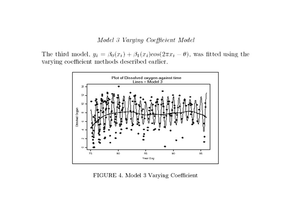
35. Example 1: water quality in the River Clyde A general varying coefficient model is of the form – y i = 0 (x i ) + 1 (x i )cos(2 x i - (x i )) + i ; i = 1;…;n; – includes a mean trend term and seasonal variation as follows: x i is year in decimal term – This includes smooth terms 0 and 1 and a varying coefficient seasonal term (modelled parametrically) – This can be simplified by setting some parameters to be constant

36. Seasonality-river Clyde

38. Example 2: Loch Leven-trends correcting for covariates Loch Leven: key loch for water framework directive: environmental effect of interest is eutrophication: measurement series covers 30 years, including a variety of biological, chemical and hydrological indicators but irregular in time. Substantial improvement in the loch water quality, – How is climate change affecting the loch and is it reasonable to expect that it can ever return to reference conditions? – Explored using additive and varying coefficient models to look at trend and climate

39. Loch Leven

40. Additive Models

41. Example 3: trends in atmospheric SO 2 levels over space- EMEP network Daily measurements made at more than 100 monitoring stations over a 20 year period over Europe: Complex statistical model developed to describe the pattern, the model portions the variation to trend, seasonality, residual variation Main question: – what is the long term trend and is it the same over Europe?

43. Additive models including space ln(SO 2 ) = f ym (years, months) + f ll (latitude, longitude) + ln(SO 2 ) = f y (years) + f m (months) + f ll (latitude, longitude) + with appropriate assumptions on

44. ln(SO 2 ) = f y (years) + f m (months) + f ll (latitude, longitude) + ln(SO 2 ) = f ym (years, months) + f ll (latitude, longitude) +

45. Measurement and assessment of change-three questions to consider Is routine monitoring data useful/adequate/sufficient for environmental change detection? Are the classical (well accepted) simple procedures such as – the % change between two time points (the slope), – A p-value or a 95% confidence interval for the slope sufficient for the complexity of environmental behaviour? What do statistical trends offer to evaluation of environmental change, to management and to policy setting? how long does a time series need to be?

46. Statistical trends and environmental change Sophisticated statistical models for trends can give – added value and better descriptions of complex change behaviour and – begin to tease out climate change driven effects in environmental quality

47. Case study: Central England temperature R script in CETcasestudy explore the trend (linear or otherwise) is the trend the same in the different months does the starting point matter in our conclusions?