1. Probability Exercises

2. Experiment Something capable of replication under stable conditions. Example: Tossing a coin

3. Sample Space The set of all possible outcomes of an experiment. A sample space can be finite or infinite, & discrete or continuous.

4. A set is discrete if you can put you finger on one element after another & not miss any in between. That’s not possible if a set is continuous.

5. Example: discrete, finite sample space Experiment: Tossing a coin once. Sample space: {H, T}. This sample space is discrete; you can put your finger on one element after the other & not miss any. This sample space is also finite. There are just two elements; that’s a finite number.

6. Example: discrete, infinite sample space Experiment: Eating potato chips: Sample space: {0, 1, 2, 3, 4, 5, 6, 7, 8, 9, 10, 11,...} This sample space is discrete; you can put your finger on one element after another & not miss any in between. This sample space is infinite, however, since there are an infinite number of possibilities.

7. Example: continuous sample space. Experiment: Burning a light bulb until it burns out. Suppose there is a theoretical maximum number of hours that a bulb can burn & that is 10,000 hours. Sample space: The set of all real numbers between 0 & 10,000. Between any two numbers you can pick in the sample space, there is another number. For example, the bulb could burn for 99.777 hours or 99.778. But it could also burn for 99.7775, which is in between. You cannot put your finger on one element after another & not miss any in between. This sample space is continuous. It is also infinite, since there are an infinite number of possibilities. All continuous sample spaces are infinite.

8. Event a subset of the outcomes of an experiment Example: Experiment: tossing a coin twice Sample space (all possible outcomes) = {HH, HT, TH, TT} An event could be that you got at least one head on the two tosses. So the event would be {HH, HT, TH}

9. Subjective versus objective probability

10. Subjective vs. Objective Probability Subjective Probability is probability in lay terms. Something is probable if it is likely. Example: I will probably get an A in this course. Objective Probability is what we’ll use in this course. Objective Probability is the relative frequency with which something occurs over the long run. What does that mean?

11. Objective Probability: Developing the Idea Suppose we flip a coin & get tails. Then the relative frequency of heads is 0/1 = 0. Suppose we flip it again & get tails again. Our relative frequency of heads is 0/2 = 0. We flip it 8 more times & get a total of 6 tails & 4 heads. The relative freq of heads is 4/10 = 0.4 We flip it 100 times & get 48 heads. The relative freq of heads is 48/100 = 0.48 We flip it 1000 times & get 503 heads. The relative freq of heads is 503/1000 = 0.503 If the coin is fair, & we could flip it an infinite number of times, what would the relative frequency of heads be? 0.5 or 1/2 That’s the relative freq over the long run or probability of heads.

12. Two Basic Properties of Probability 1. 0 < Pr(E) < 1 for every subset of the sample space S 2. Pr(S) = 1

13. Counting Rules We’ll look at three counting rules. – 1. Basic multiplication rule – 2. Permutations – 3. Combinations

14. Multiplication Rule Example

15. Suppose we toss a coin 3 times & examine the outcomes. (One possible outcome would be HTH.) How many outcomes are possible?

16. We have 2 possibilities for the 1st toss, H & T. H T

17. We can pair each of these with 2 possibilities. H T H T H T

18. That gives 4 possibilities on the 2 tosses: HH, H T H T H T

19. HT, H T H T H T

20. TH H T H T H T

21. And TT H T H T H T

22. If we toss the coin a 3rd time, we can pair each of 4 possibilities with a H or T. H T H T H T H T H T H T H T

23. So for 3 tosses, we have 8 possibilities: HHH, H T H T H T H T H T H T H T

24. HHT, H T H T H T H T H T H T H T

25. HTH, H T H T H T H T H T H T H T

26. HTT, H T H T H T H T H T H T H T

27. THH, H T H T H T H T H T H T H T

28. THT, H T H T H T H T H T H T H T

29. TTH, H T H T H T H T H T H T H T

30. and TTT. H T H T H T H T H T H T H T

31. Again, we had 8 possibilities for 3 tosses. 2 x 2 x 2 = 2 3 = 8

32. In general, If we have an experiment with k parts (such as 3 tosses) and each part has n possible outcomes (such as heads & tails), then the total number of possible outcomes for the experiment is n k n k This is the simplest multiplication rule.

33. As a variation, suppose that we have an experiment with 2 parts, the 1st part has m possibilities, & the 2nd part has n possibilities. How many possibilities are there for the experiment?

34. In particular, we might have a coin & a die. So one possible outcome could be H6 (a head on the coin & a 1 on the die). How many possible outcomes does the experiment have?

35. We have 2 x 6 = 12 possibilities. Return to our more general question about the 2-part experiment with m & n possibilities for each part. We now see that the total number of outcomes for the experiment is mn

36. If we had a 3-part experiment, the 1st part has m possibilities, the 2nd part has n possibilities, & the 3rd part has p possibilities, how many possible outcomes would the experiment have? m n p

37. Permutations Counting Rules

38. Permutations Suppose we have a horse race with 8 horses: A,B,C,D,E,F,G, and H. We would like to know how many possible arrangements we can have for the 1st, 2nd, & 3rd place horses. One possibility would be G D F. (F D G would be a different possibility because order matters here.)

39. We have 8 possible horses we can pick for 1st place. Once we have the 1st place horse, we have 7 possibilities for the 2nd place horse. Then we have 6 possibilities for the 3rd place horse. So we have 8 7 6 = 336 possibilities. This is the number of permutations of 8 objects (horses in this case), taken 3 at a time.

40. How many possible arrangements of all the horses are there? In other words, how many permutations are there of 8 objects taken 8 at a time? 8 7 6 5 4 3 2 1 = 40,320 This is 8 factorial or 8!

41. We’d like to develop a general formula for the number of permutations of n objects taken k at a time. Let’s work with our horse example of 8 horses taken 3 at a time. The number of permutations was 8 7 6.

42. We can multiply our answer (8 7 6) by 1 & still have the same answer. Note that this is Multiplying we have

43. So the number of permutations of n objects taken k at a time is

44. Combinations Counting Rules

45. Combinations Suppose we want to know how many different poker hands there are. In other words, how many ways can you deal 52 objects taken 5 at a time. Keep in mind that if we have 5 cards dealt to us, it doesn’t matter what order we get them. It’s the same hand. So while order matters in permutations, order does not matter in combinations.

46. Let’s start by asking a different question. What is the number of permutations of 52 cards taken 5 at a time? n P k = 52 P 5 = 52 51 50 49 48 = 311,875,200 When we count the number of permutations, we are counting each reordering separately.

47. However, each reordering should not be counted separately for combinations. We need to figure out how many times we counted each group of 5 cards. For example, we counted the cards ABCDE separately as ABCDE, BEACD, CEBAD, DEBAC, etc. How many ways can we rearrange 5 cards? We could rearrange 8 horses 8! ways. So we can rearrange 5 cards 5! = 120 ways.

48. That means that we counted each group of cards 120 times. So the number of really different poker hands is the number of permutations of 52 cards taken 5 at a time divided by the 120 times that we counted each hand.

49. So the number of combinations of 52 cards taken 5 at a time is

50. The number of combinations of n objects taken k at a time is

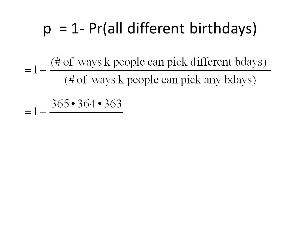
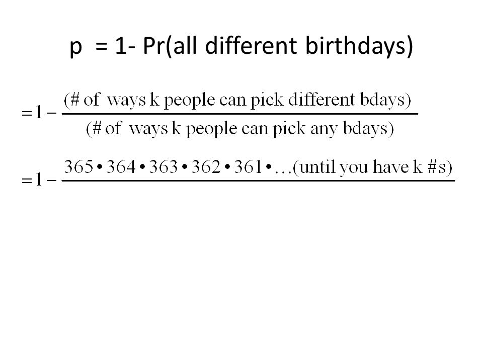
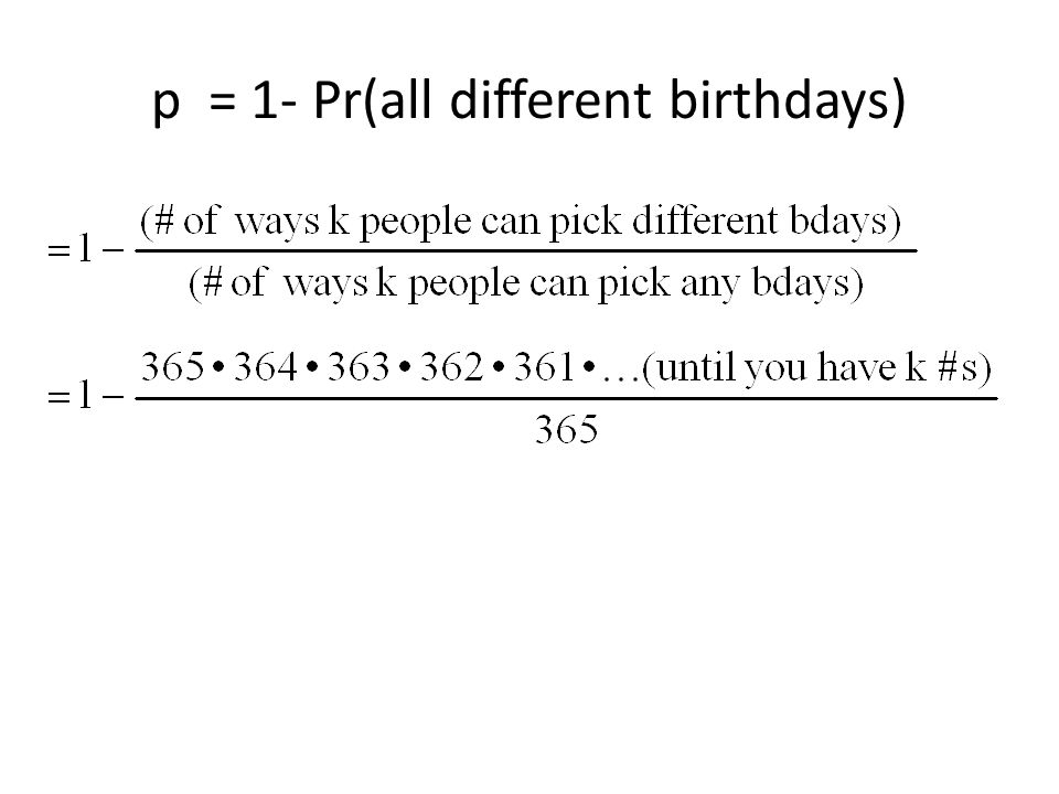
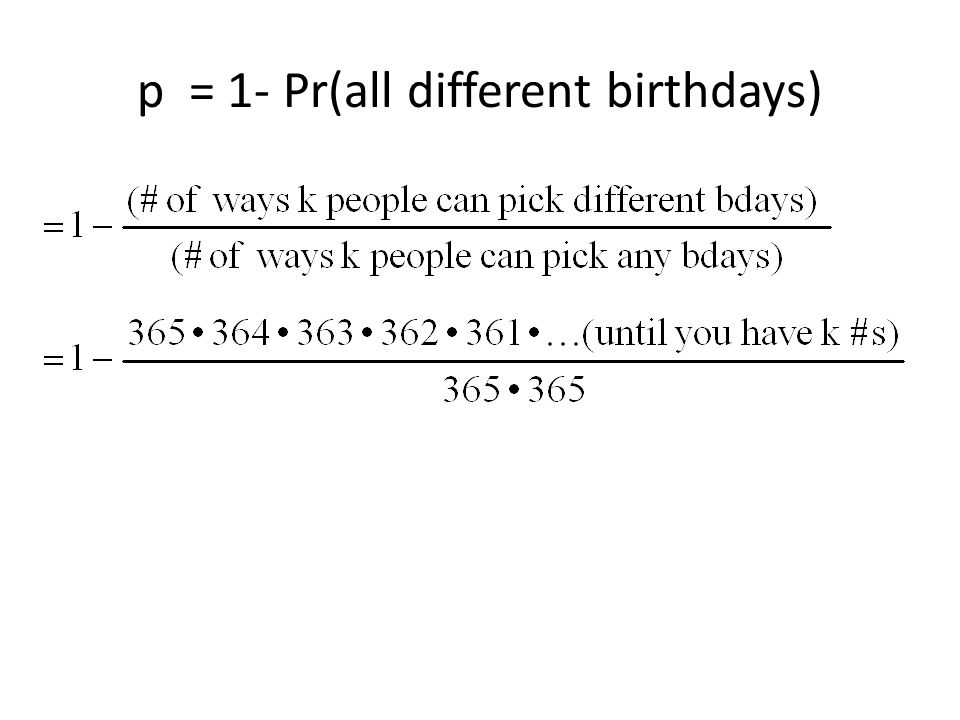
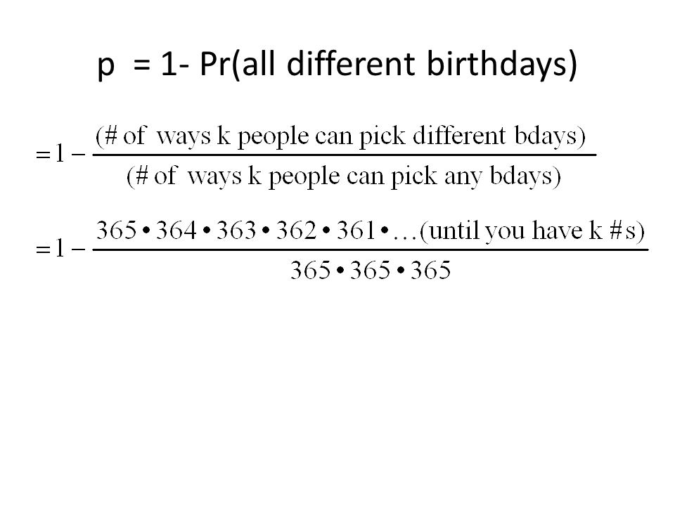
51. The number of combinations of n objects taken k at a time n C k is also written as n k and is read as “n choose k”. It’s the number of ways you can start with n objects and choose k of them without regard to order.

52. Complements, Unions, & Intersections Suppose A & B are events.

53. The complement of A is everything in the sample space S that is NOT in A. If the rectangular box is S, and the white circle is A, then everything in the box that’s outside the circle is A c, which is the complement of A. A S

54. Theorem Pr (A c ) = 1 - Pr (A) Example: If A is the event that a randomly selected student is male, and the probability of A is 0.6, what is A c and what is its probability? A c is the event that a randomly selected student is female, and its probability is 0.4.

55. The union of A & B (denoted A U B) is everything in the sample space that is in either A or B or both. The union of A & B is the whole white area. A S B

56. The intersection of A & B (denoted A∩B) is everything in the sample space that is in both A & B. The intersection of A & B is the pink overlapping area. S B A

57. Example A family is planning to have 2 children. Suppose boys (B) & girls (G) are equally likely. What is the sample space S? S = {BB, GG, BG, GB}

58. Example continued If E is the event that both children are the same sex, what does E look like & what is its probability? E = {BB, GG} Since boys & girls are equally likely, each of the four outcomes in the sample space S = {BB, GG, BG, GB} is equally likely & has a probability of 1/4. So Pr(E) = 2/4 = 1/2 = 0.5

59. Example cont’d: Recall that E = {BB, GG} & Pr(E)=0.5 What is the complement of E and what is its probability? E c = {BG, GB} Pr (E c ) = 1- Pr(E) = 1 - 0.5 = 0.5

60. Example continued If F is the event that at least one of the children is a girl, what does F look like & what is its probability? F = {BG, GB, GG} Pr(F) = 3/4 = 0.75

61. Recall: E = {BB, GG} & Pr(E)=0.5 F = {BG, GB, GG} & Pr(F) = 0.75 What is E∩F? {GG} What is its probability? 1/4 = 0.25

62. Recall: E = {BB, GG} & Pr(E)=0.5 F = {BG, GB, GG} & Pr(F) = 0.75 What is the EUF? {BB, GG, BG, GB} = S What is the probability of EUF? 1 If you add the separate probabilities of E & F together, do you get Pr(EUF)? Let’s try it. Pr(E) + Pr(F) = 0.5 + 0.75 = 1.25 ≠ 1 = Pr (EUF) Why doesn’t it work? We counted GG (the intersection of E & F) twice.

63. A formula for Pr(EUF) Pr(EUF) = Pr(E) + Pr(F) - Pr(E∩F) If E & F do not overlap, then the intersection is the empty set, & the probability of the intersection is zero. When there is no overlap, Pr(EUF) = Pr(E) + Pr(F).

64. Conditional Probability of A given B Pr(A|B) Pr(A|B) = Pr (A∩B) / Pr(B)

65. Example Example Suppose there are 10,000 students at a university. 2,000 are seniors (S). 3,500 are female (F). 800 are seniors & female. Determine the probability that a randomly selected student is (1) a senior, (2) female, (3) a senior & female. 1. Pr(S) = 2,000/10,000 = 0.2 2. Pr(F) = 3,500/10,000 = 0.35 3. Pr(S∩F) = 800/10,000 = 0.08

66. Use the definition of conditional probability Pr(A|B) = Pr(A∩B) / Pr(B) & the previously calculated information Pr(S) = 0.2; Pr(F) = 0.35; Pr(S∩F) = 0.08 to answer the questions below. 1. If a randomly selected student is female, what is the probability that she is a senior? Pr(S|F) = Pr(S∩F) / Pr(F) = 0.08 / 0.35 = 0.228 2. If a randomly selected student is a senior, what is the probability the student is female? Pr(F|S) = Pr(F∩S) / Pr(S) = 0.08 / 0.2 = 0.4 Notice that S∩F = F∩S, so the numerators are the same, but the denominators are different.

67. Joint Probability Distributions & Marginal Distributions

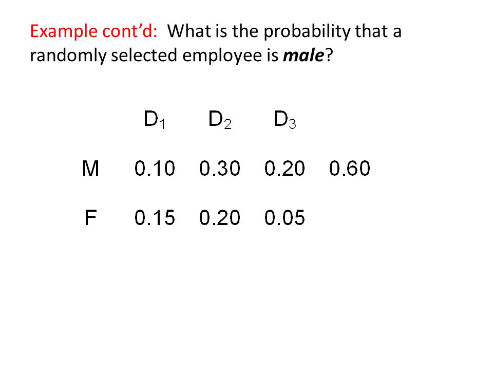
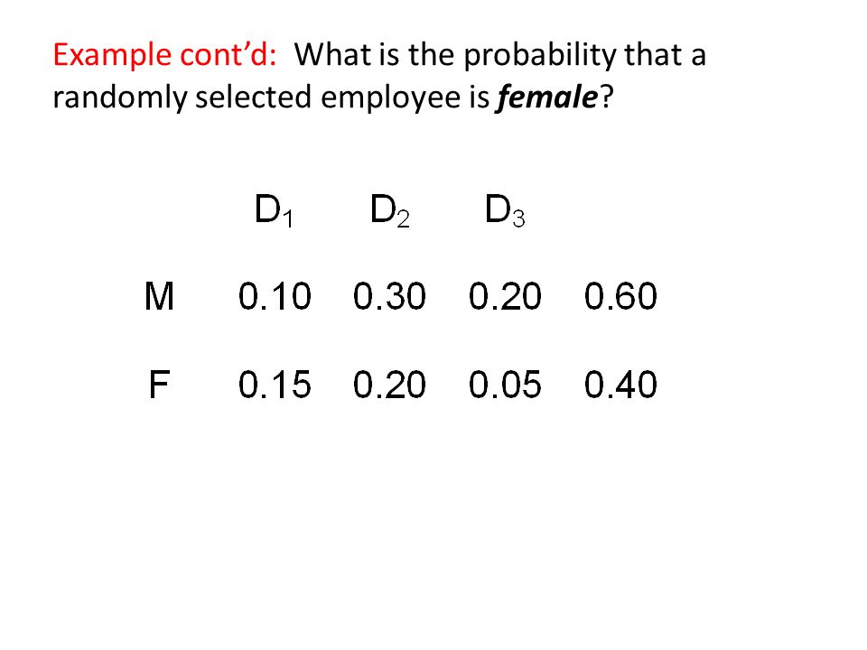
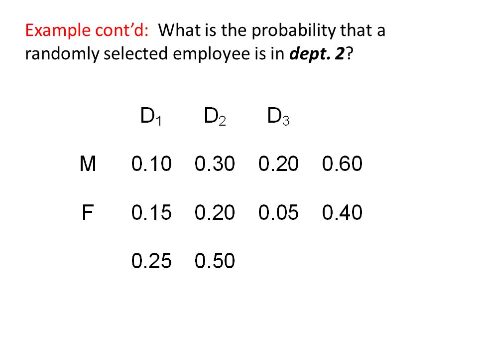
68. Example: Example: Suppose a firm has 3 departments. Of the firm’s employees, 10% are male & in dept. 1, 30% are male & in dept. 2, 20% are male & in dept. 3, 15% are female & in dept. 1, 20% are female & in dept. 2, & 5% are female & in dept. 3. Then the joint probability distribution of gender & dept. is as in the table below.

69. Example cont’d: What is the probability that a randomly selected employee is male?

71. Example cont’d: What is the probability that a randomly selected employee is female?

73. Example cont’d: What is the probability that a randomly selected employee is in dept. 1?

75. Example cont’d: What is the probability that a randomly selected employee is in dept. 2?

77. Example cont’d: What is the probability that a randomly selected employee is in dept. 3?

79. Example cont’d: The marginal distribution of gender is in first & last columns (or left & right margins of the table) & gives the probability of each possibility for gender.

80. Example cont’d: The marginal distribution of department is in first & last rows (or top & bottom margins of the table) & gives the probability of each possibility for dept.

81. Notice that when you add the numbers in the last column or the last row, you must get one, because you’re adding all the probabilities for all the possibilities.

82. Bayesian Analysis Allows us to calculate some conditional probabilities using other conditional probabilities

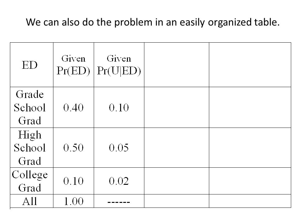
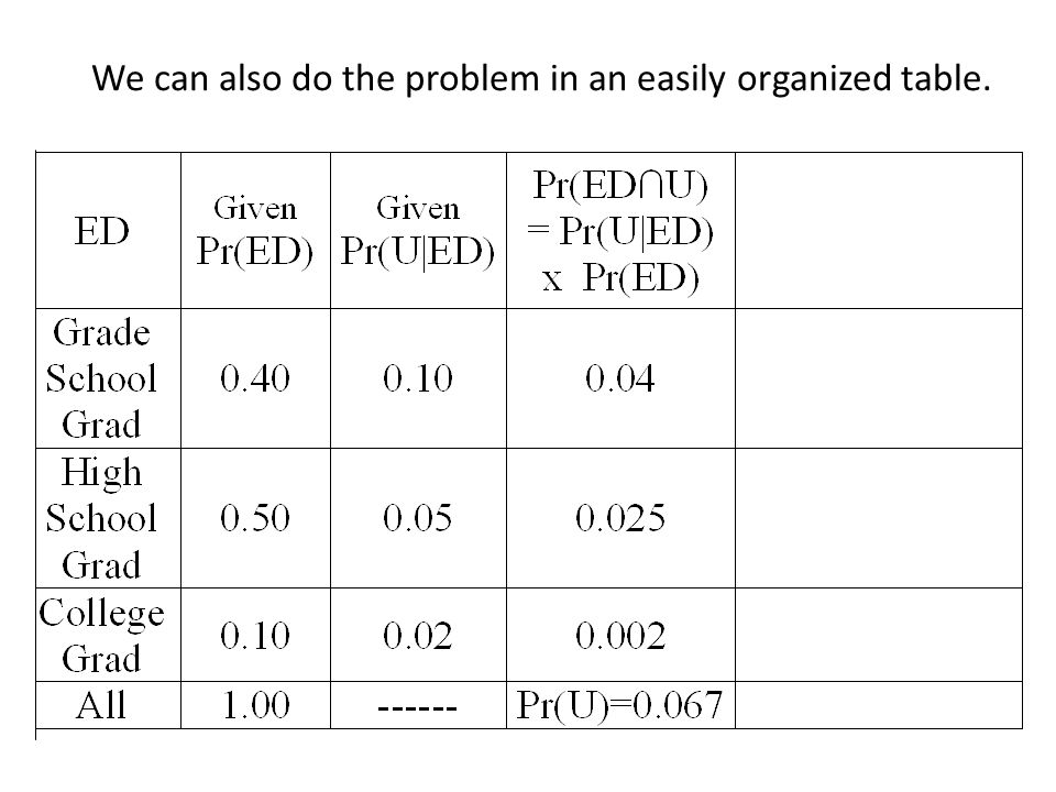
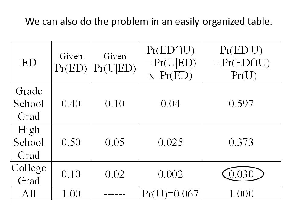
83. Example: We have a population of potential workers. We know that 40% are grade school graduates (G), 50% are high school grads (H), & 10% are college grads (C). In addition, 10% of the grade school grads are unemployed (U), 5% of the h.s. grads are unemployed (U), & 2% of the college grads are unemployed (U). Convert this information into probability statements. Then determine the probability that a randomly selected unemployed person is a college graduate, that is, Pr(C|U).

84. 40% are grade school graduates (G), 50% are high school grads (H), & 10% are college grads (C). In addition, 10% of the grade school grads are unemployed (U), 5% of the h.s. grads are unemployed (U), & 2% of the college grads are unemployed (U). Pr(G) = 0.40

85. 40% are grade school graduates (G), 50% are high school grads (H), & 10% are college grads (C). In addition, 10% of the grade school grads are unemployed (U), 5% of the h.s. grads are unemployed (U), & 2% of the college grads are unemployed (U). Pr(G) = 0.40 Pr(H) = 0.50

86. 40% are grade school graduates (G), 50% are high school grads (H), & 10% are college grads (C). In addition, 10% of the grade school grads are unemployed (U), 5% of the h.s. grads are unemployed (U), & 2% of the college grads are unemployed (U). Pr(G) = 0.40 Pr(H) = 0.50 Pr(C) = 0.10

87. 40% are grade school graduates (G), 50% are high school grads (H), & 10% are college grads (C). In addition, 10% of the grade school grads are unemployed (U), 5% of the h.s. grads are unemployed (U), & 2% of the college grads are unemployed (U). Pr(G) = 0.40Pr(U|G) = 0.10 Pr(H) = 0.50 Pr(C) = 0.10

88. 40% are grade school graduates (G), 50% are high school grads (H), & 10% are college grads (C). In addition, 10% of the grade school grads are unemployed (U), 5% of the h.s. grads are unemployed (U), & 2% of the college grads are unemployed (U). Pr(G) = 0.40Pr(U|G) = 0.10 Pr(H) = 0.50Pr(U|H) = 0.05 Pr(C) = 0.10

89. 40% are grade school graduates (G), 50% are high school grads (H), & 10% are college grads (C). In addition, 10% of the grade school grads are unemployed (U), 5% of the h.s. grads are unemployed (U), & 2% of the college grads are unemployed (U). Pr(G) = 0.40Pr(U|G) = 0.10 Pr(H) = 0.50Pr(U|H) = 0.05 Pr(C) = 0.10Pr(U|C) = 0.02

90. In order to calculate Pr(C|U), we need to determine the probability that a randomly selected individual is 1. a grade school grad & unemployed 2. a h.s. grad & unemployed 3. a college grad & unemployed

91. Then 10% of 40% of our population is grade school grads & unemployed. So Pr(G & U) = Pr(G∩U) = 0.10 x 0.40 = 0.04. Similarly, Pr(H & U) = Pr(H∩U) = 0.05 x 0.50 = 0.025. Also, Pr(C & U) = Pr(C∩U) = 0.02 x 0.10 = 0.002. Recall that 40% of our population is grade school grads, & 10% of them are unemployed.

92. Pr(U) = Pr(G∩U) + Pr(H∩U) + Pr(C∩U) = 0.04 + 0.025 + 0.002 = 0.067 Given Pr(G & U) = Pr(G ∩ U) = 0.04, Pr(H & U) = Pr(H ∩ U) = 0.025, & Pr(C & U) = Pr(C ∩ U) = 0.002, we can calculate the probability that a randomly selected individual is unemployed, Pr(U).

93. We can finally determine Pr(C|U), using our calculations & the definition of conditional probability. Pr(C|U) = Pr(C∩U) / Pr(U) = 0.002 / 0.067 = 0.030. So the probability that a randomly selected unemployed individual is a college graduate is 0.03.

94. We can also do the problem in an easily organized table.

98. Independence Two events are independent, if knowing that one event happened doesn’t give you any information on whether the other happened. Example: A: It rained a lot in Beijing, China last year. B: You did well in your courses last year. These two events are independent (unless you took your courses in Beijing). One of these events occurring tells you nothing about whether the other occurred.

99. So in terms of probability, two events A & B are independent if and only if * Pr(A|B) = Pr(A) Using the definition of conditional probability, this statement is equivalent to Pr(A∩B) / Pr(B) = Pr(A). Multiplying both sides by Pr(B), we have * Pr(A∩B) = Pr(A) Pr(B). Dividing both sides by Pr(A), we have Pr(A∩B) / Pr(A) = Pr(B), which is equivalent to * Pr(B|A) = Pr(B). This makes sense. If knowing about B tells us nothing about A, then knowing about A tells us nothing about B.

100. We now have 3 equivalent statements for 2 independent events A & B Pr(A|B) = Pr(A) Pr(B|A) = Pr(B) Pr(A ∩ B) = Pr(A) Pr(B). The last equation says that you can calculate the probability that both of two independent events occurred by multiplying the separate probabilities.

101. Example: Toss a fair coin & a fair die A: You get a H on the coin. B: You get a 6 on the die. Recall that we counted 12 possible outcomes for this experiment. Since the coin & the die are fair, each outcome is equally likely, & the probability of getting a H & a 6 is 1/12.

102. Example cont’d The probability of a H on the coin is 1/2 The probability of a 6 on the die is 1/6. So Pr(H) Pr(6) = (1/2)(1/6) = 1/12 = Pr(H ∩ 6), & we can see that these 2 events are independent of each other.

103. Mutually Exclusive Two events are mutually exclusive if you know that one occurred, then you know that the other could not have occurred. example: You selected a student at random. A: You picked a male. B: You picked a female. These 2 events are mutually exclusive, because you know that if A occurred, B did not.

104. Mutually exclusive events are NOT independent! Remember that for independent events, knowing that one event occurred tells you nothing about whether the other occurred. For mutually exclusive events, knowing that one event occurred tells you that the other definitely did not occur!

105. The Birthday Problem

106. What is the probability that in a group of k people at least two people have the same birthday? (We are going to ignore leap day, which complicates the analysis, but doesn’t have much effect on the answer.)

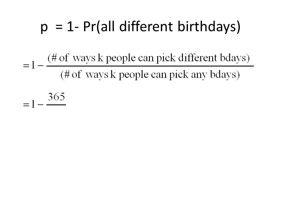
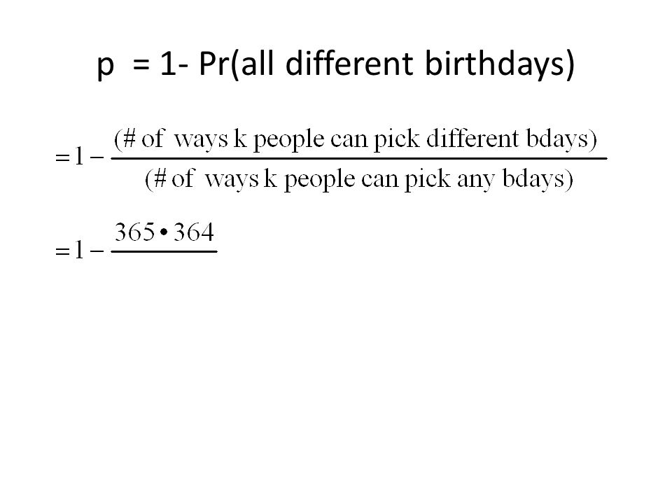
107. For our group of k people, let p = Pr(at least 2 people have the same birthday). At least 2 people having the same birthday is the complement (opposite) of no 2 people having the same birthday, or everyone having different birthdays. It’s easier to calculate the probability of different birthdays. So we can do that & then subtract the answer from one to get the probability we want.

108. p = 1- Pr(all different birthdays)

116. This is very messy, but you can calculate the answer for any number k. I have the answers computed for some sample values.

117. Birthday Problem Probabilities k p 50.027 100.117 150.253 200.411 220.476 230.507 250.569 300.706 400.891 500.970 1000.9999997