Download presentation
Presentation is loading. Please wait.

1
NUMERICAL INVESTIGATION OF STEADY WEAR PROCESS Páczelt István University of Miskolc, Department of Mechanics, Miskolc, Hungary 2-nd Hungarian-Ukrainian Joint Conference on SAFETY-RELIABILITY AND RISK OF ENGINEERING PLANTS AND COMPONENTS KYIV, September 19-21, 2007.

2
A contact problem

3
Linear elastic contact problems Contact conditions

4
Signorini contact conditions Friction conditions: In adhesion subregion In slip subregion

5
Contact stresses

6
Clasification of mechanical wear processes

7
Factors influencing dry wear rates

8
Modified Archard wear model

9
Problem classification 1. Rigid body wear velocities allowed, contact area fixed- steady states present

10
2.Rigid body wear velocities allowed, contact area evolving in time due to wear- quasi steady states

11
3.No rigid body wear velocities allowed- steady states corresponding to vanishing wear rate and contact pressure (wear shake down).
.")
12
Initial gap g= g_0 =0.05 mm, Beam side a_0=10 mm, b_0=25 mm, lenght L=300 mm. Load F_0=10 kN, AB distance (a) =150mm, Relative velocity v_r=50 mm/s Coefficient of Winkler foundation= 0.0000002 mm/N
 =150mm, Relative velocity v_r=50 mm/s Coefficient of Winkler foundation= mm/N.")
13
The wear parameters are: beta=0.0025, a=b=1 coefficient of friction mu=0.3 In initial state: (u1_n beam displacement in vertical direction without body 2.) def1, def2 are vertical displacement of body 1 and 2 in the contact.
 def1, def2 are vertical displacement of body 1 and 2 in the contact.")
14
Initial state:

15
In the time t=0.8 sec

16
In the time t=1200*dt=1200*0.001=1,2 sec

17
In the time t=2,4 sec

18
In the time= 3,6 sec

19
In the time= 7,8 sec

20
In the time=12 sec

21
In the time=60 sec Here p_n= 1*10e-7 that is practically p_n is equal to zero.

22
4. Oscillating sliding contacts (fretting process)
")
23
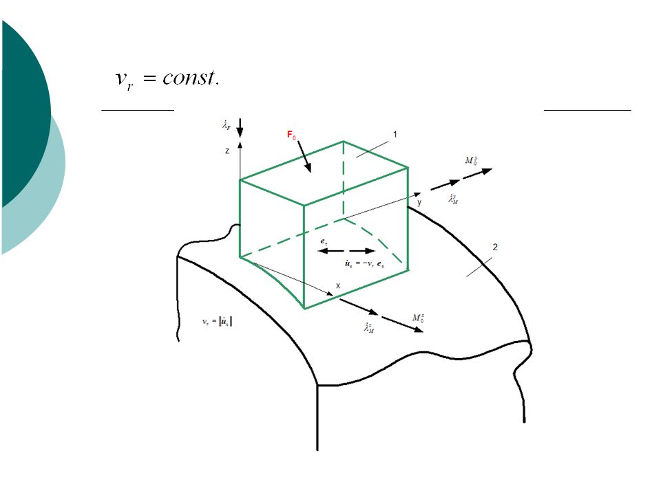
Type of investigated mechanical systems The analysis of the present investigation is referred to such class of problems when the contact surface does not evolve in time and is specified the wear velocity associated with rigid body motion does not vanish and is compatible with the specified boundary conditions

24
[1] Páczelt I, Mróz Z. On optimal contact shapes generated by wear, Int. J. Num. Meth. Eng. 2005;63:1310-1347. [2] Páczelt I, Mróz Z. Optimal shapes of contact interfaces due to sliding wear in the steady relative motion, Int. J. Solids Struct 2007;44:895-925. [3] Pödra P, Andersson S. Simulating sliding wear with finite element method, Tribology Int 1999;32:71-81. [4] Öqvist M. Numerical simulations of mild wear using updated geometry with different step size approaches, Wear 2001;49:6- 11. [5] Peigney U. Simulating wear under cyclic loading by a minimization approach, Int. J. Solids Struct 2004;41: 6783-6799. [6] Marshek KM, Chen HH. Discretization pressure wear theory for bodies in sliding contact, J. Tribology ASME 1989; 111:95- 100. [7] Sfantos GK, Aliabadi MH. Application of BEM and optimization technique to wear problems, Int. J. Solids Struct 2006;43:3626- 3642. [8] Kim NH, Won D, Burris D, Holtkamp B, Gessel GC, Swanson P, Sawyer WG. Finite element analysis and experiments of metal/metal wear in oscillatory contacts, Wear 2005;258:1787- 1793. [9] Fouvry S. et al. An energy description of wear mechanisms and its applications to oscillating sliding contacts, Wear, 2003;255:287-298
![ [1] Páczelt I, Mróz Z. On optimal contact shapes generated by wear, Int.](http://images.slideplayer.com/25/7676391/slides/slide_24.jpg "J. Num. Meth. Eng. 2005;63: [2] Páczelt I, Mróz Z. Optimal shapes of contact interfaces due to sliding wear in the steady relative motion, Int. J. Solids Struct 2007;44: [3] Pödra P, Andersson S. Simulating sliding wear with finite element method, Tribology Int 1999;32: [4] Öqvist M. Numerical simulations of mild wear using updated geometry with different step size approaches, Wear 2001;49: [5] Peigney U. Simulating wear under cyclic loading by a minimization approach, Int. J. Solids Struct 2004;41: [6] Marshek KM, Chen HH. Discretization pressure wear theory for bodies in sliding contact, J. Tribology ASME 1989; 111: [7] Sfantos GK, Aliabadi MH. Application of BEM and optimization technique to wear problems, Int. J. Solids Struct 2006;43: [8] Kim NH, Won D, Burris D, Holtkamp B, Gessel GC, Swanson P, Sawyer WG. Finite element analysis and experiments of metal/metal wear in oscillatory contacts, Wear 2005;258: [9] Fouvry S. et al. An energy description of wear mechanisms and its applications to oscillating sliding contacts, Wear, 2003;255:")
25
The generalized wear volume rate Generalized friction dissipation power

26
The generalized wear dissipation power For one body For two bodies q>0 where the control parameter q usually is

27
The relative tangential velocity on sliding velocity at the interface wear velocity are the relative translation and rotation velocities induced by wear

29
The generalized wear dissipation power Wear rate vectors:. Relative velocity:

30
The global equilibrium conditions for body 1 are

32
Constrained minimization Problem PW1: Min Problem PW2: Min Problem PW3: Min subject to

33
Major results of our investigation: Question: What kind of minimization problem generates contact pressure distribution corresponding to the steady wear state? Answer: Must be used: min

34
Main assumption: We shall consider only the generalized wear dissipation power and the resulting optimal pressure distribution. It will be shown that for q=1, the optimal solution corresponds to steady state condition.

35
Congruency conditions In stationary translation motion: In rotation with constant angular velocity: the case of annular punch:

36
Introducing the Lagrange multipliers and The Lagrangian functional is

37
From the stationary condition we obtain The equations are highly nonlinear !

38
Special case 1 the contact pressure is the wear rate equals the wear volume rate is

39
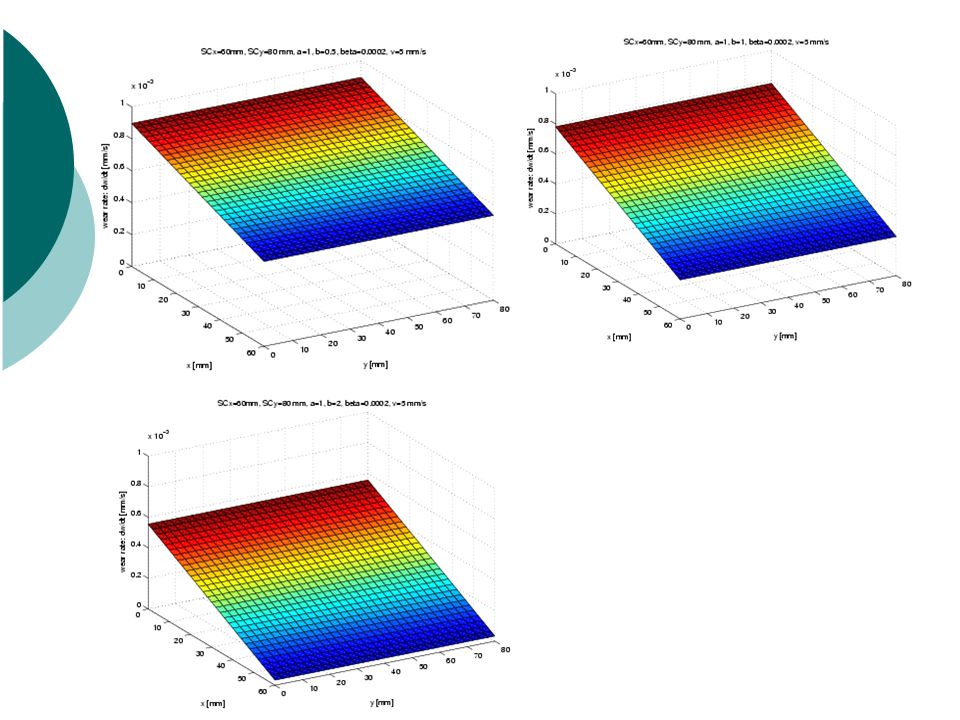
Special case 2: translation and rotation SCx=60 mm, SCy=80 mm

42
Special case 3: Block-on-disk wear tests

43
Results At steady wear state (q=1)
")
44
Contact pressure distribution for anticlockwise disk rotation

45
Vertical wear rate distribution for clockwise disk rotation

46
Normal contact shape for different values of friction coefficient, q=1

47
Vertical contact shape for different values of friction coefficient, q=1

48
Steady state normal and vertical wear rate distributions

49
Special case 4: ring segment-on- disk wear tests.

50
Initial contact pressure distribution (anticlockwise rotation).
.")
51
Optimal contact vertical shape at anticlockwise rotation

52
Special case 5: brake system with rotating block

53
Results at steady state (q=1)
")
54
Special case 6 : brake system with translating and rotating block

55
Results

56
The non-linear equations are solved by Newton-Ralphson technique At steady state,,.

57
Numerical results:pressure distribution

58
Pressure distribution

59
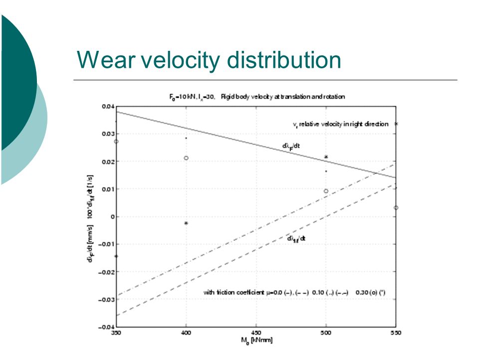
Wear velocity distribution

61
Special case 7: Automative Braking system

62
Drum brake

63
Model of drum brake

64
Equilibrium equation, wear rate vector ----------------------------------------------

65
Pressure and wear rate At steady wear state (q=1)
")
66
Optimal contact pressure distribution at anticlockwise drum rotation

67
Optimal contact pressure distribution:clockwise drum rotation

68
Wear rate distributions in the steady state: q=1, (anticlockwise drum rotation)
")
69
Wear rate distributions in the steady state: q=1, (clockwise drum rotation)
")
70
Special case 8: Cylindrical punch rotation with respect to symmetry axis

71
Contact pressure, Lagrangian functional

72
At steady state (q=1) Contact pressure Vertical wear rate
 Contact pressure Vertical wear rate")
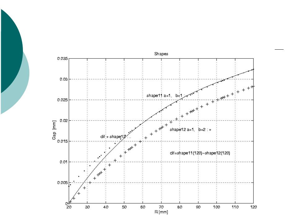
73
Distribution of contact pressure

74
Vertical gap at steady state

75
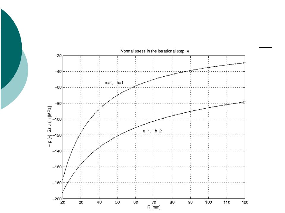
Stress state in body B1

76
If then the contact surface will be a plate

77
Contact pressure for different wear parameters

78
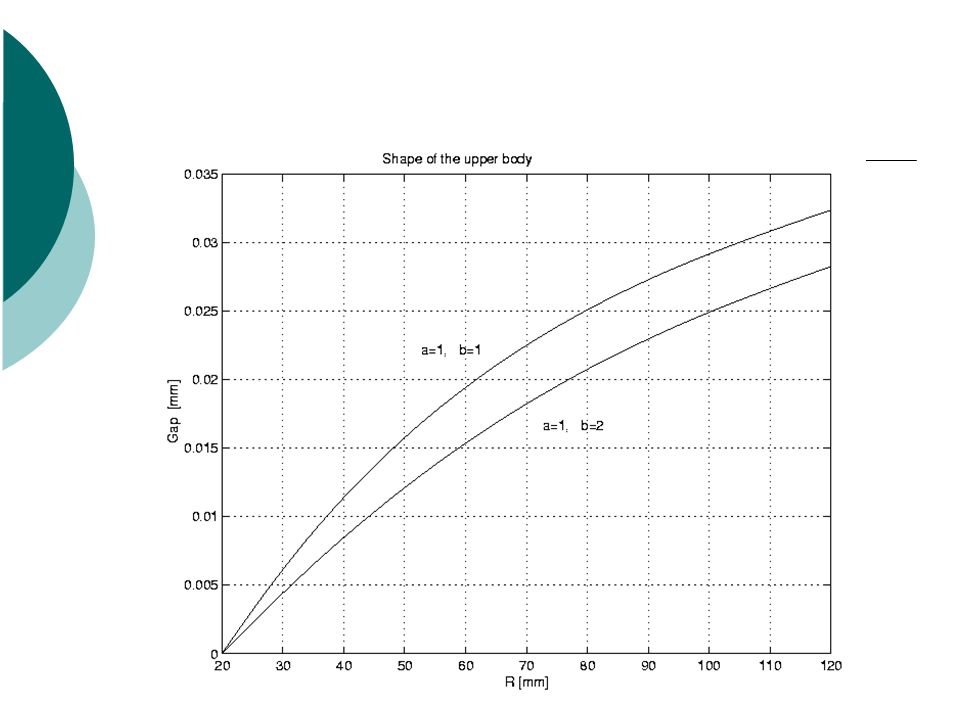
Contact shape in the steady state

79
Initial shape calculated for The wear process for the system Time step:

83
DeltaV= V(i)-V(i-1) - (V(i-1)-V(i-2)), i=2,3,4,….
-V(i-1) - (V(i-1)-V(i-2)), i=2,3,4,….")
84
The wear shape in the different time step

85
Effect of heat generation

86
Shape in steady wear state a) without temperature, b) with influence of heat generation
 without temperature, b) with influence of heat generation")
87
Special case 9: disk brake

88
Model of disk brake

89
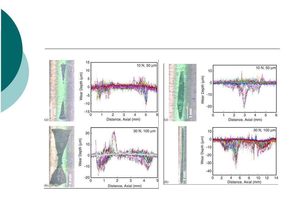
Special case 10: Nuclear fuel fretting

90
Procedure to solve wear problem in the industry.

91
Kim: Tribology International, 36 (2006), p.1305-1319
, p")
95
M. Helmi Attia: Tribology International, 39 (2006), p. 1294-1304.
, p")
96
Heat exchanger tube

97
System approach to the fretting wear process

98
Conclusions 1.The present lecture provides a uniform approach to the analysis of steady wear regimes developing in the case of sliding relative motion of contacting bodies. 2. Usually, the steady state may be attained experimentally or in the numerical analysis by integrating the wear rate in the transient wear period. 3. A fundamental assumption is now introduced, namely, at the steady state the wear rate vector is collinear with the rigid body wear velocity of body 1. 4. The minimum of the generalized wear dissipation power for q = 1 generates steady state regimes.

99
Conclusions: 5. The optimal solution corresponds to steady state condition. Thus, this condition can be specified directly from formulae for contact pressure and equilibrium equations instead of integration of the wear rule for whole transient wear process until the steady state is reached. 6. The specification of steady wear states is of engineering importance as it allows for optimal shape design of contacting interfaces in order to avoid the transient run-in periods. 7. Different numerical examples demonstrate usefulness of the proposed principle and corresponding numerical methods. 8. High accuracy solution may be reached using the p- version of finite elements for the contact problems combined with the positioning technique and the special remeshing.

100
Closure Thank you very much for your kind attention!

Similar presentations


>")


 St. Petersburg Polytechnical University Author:>")


