Download presentation
Presentation is loading. Please wait.

1
Computational Issues: An EnKF Perspective Jeff Whitaker NOAA Earth System Research Lab ENIAC 1948“Roadrunner” 2008

2
EnKF cycle 1)Run ensemble forecast for each ensemble member to get x b for next analysis time. 2)Compute Hx b for each ensemble member. 3)Given Hx b, x b compute analysis increment (using LETKF, EnSRF etc)
Compute Hx b for each ensemble member. 3)Given Hx b, x b compute analysis increment (using LETKF, EnSRF etc).")
3
EnKF Cycle (2)
")
4
Step 1: Background Forecast 4DVar - a single run of the (high-res) non- linear forecast model for each outer loop, many runs of (low-res) TLM/adjoint in inner loop in sequence. EnKF - N simultaneous runs of the non-linear forecast model (embarassingly parallel). Bottom line - total cost similar, but EnKF may scale better.
. Bottom line - total cost similar, but EnKF may scale better..")
5
Step 2: Forward operator 4DVar - compute full nonlinear Hx b in each outer loop. In each inner loop, use linearized H (faster, especially for radiances). EnKF - compute full nonlinear Hx b once for each ensemble member simultaneously. Could use linearized H for ensemble perturbations. Bottom line - total cost similar, but EnKF may be scale better.
. EnKF - compute full nonlinear Hx b once for each ensemble member simultaneously. Could use linearized H for ensemble perturbations. Bottom line - total cost similar, but EnKF may be scale better..")
6
Step 3: Calculating the increment For EnKF, depends on algorithm –Perturbed obs EnKF (Env. Canada - obs processed serially in batches) ? –Local Ensemble Transform KF (LETKF - developed at U. of Md, being tested at JMA and NOAA) –Serial Ensemble Square-Root Filter (EnSRF - NCAR’s DART, NOAA ESRL, UW real-time WRF)
 . –Local Ensemble Transform KF (LETKF - developed at U. of Md, being tested at JMA and NOAA) –Serial Ensemble Square-Root Filter (EnSRF - NCAR’s DART, NOAA ESRL, UW real-time WRF).")
7
Serial EnSRF algorithm Whitaker and Hamill, 2002: MWR, 130, 1913-1924 Anderson, 2003: MWR, 131, 634-642 Assume ob errors uncorrelated (R diagonal). Loop over all L obs (m=1,…L). K = Ens. size 1)Update N loc ‘nearby’ state variables with this observation. Covariance (P b H T ) costs O(K* N loc ) 2)Update L loc -m ‘nearby’ observation priors (for obs not yet processed) with this observation. Covariance (HP b H T ) costs O(K*(L loc -m)) Total cost estimate O(K*L*N loc ) + O(K*L*L loc ) where L loc =av. # of ‘nearby’ ob priors and N loc =av. # of ‘nearby state elements (for each ob).
. K = Ens. size 1)Update N loc ‘nearby’ state variables with this observation. Covariance (P b H T ) costs O(K* N loc ) 2)Update L loc -m ‘nearby’ observation priors (for obs not yet processed) with this observation. Covariance (HP b H T ) costs O(K*(L loc -m)) Total cost estimate O(K*L*N loc ) + O(K*L*L loc ) where L loc =av. # of ‘nearby’ ob priors and N loc =av. # of ‘nearby state elements (for each ob)..")
8
EnSRF parallel implementation Anderson and Collins, 2007: Journal of Atmospheric and Oceanic Technology A, 24 1452-1463 Update subset of model state and observation priors on each processor. Loop over all obs on each processor - get ob priors from processor on which it is updated via MPI_Bcast of K values.

9
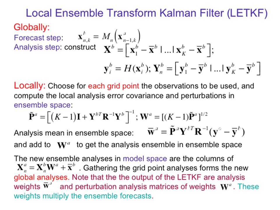
LETKF Algorithm Ob error in local volume is increased as a function of distance from red dot, reaching infinity at edge of circle.

10
LETKF cost estimate (Szyunogh et al 2008: Tellus, 60A, 113-130) Each state variable can be updated independently (perfectly parallel, no communication needed). Assume diagonal R. Most expensive step is Y b R -1 Y bT, where Y is K x L loc matrix of observation priors. L loc is average number of obs in each local region. Cost is O(K 2 *L loc *N) vs O(K* L*N loc ) + O(K*L*L loc ) for EnSRF (neglecting communication cost) –For L <= N, EnSRF faster –For L > K*N, LETKF faster –For N~L, LETKF is should be about O(K*L local /L) slower.
 vs O(K* L*N loc ) + O(K*L*L loc ) for EnSRF (neglecting communication cost) –For L <= N, EnSRF faster –For L > K*N, LETKF faster –For N~L, LETKF is should be about O(K*L local /L) slower..")
11
Benchmarks Compares only cost of computing increment (no I/O, no forward operator). 2100 km, 1.5 scale height localization, K=64 ensemble members. Two cases: –384x190 (T126) analysis grid, two tracers updated. N=23420160, L=33301. –128x64 analysis grid, no tracers updated. N=449820, L=949352. 8 core intel cluster, infiniband, mvapich2, intel fortran 10.1/MKL. Load balancing using “Graham’s algorithm” - assign each grid pt to processor with least work assigned so far.
 analysis grid, two tracers updated. N= , L= –128x64 analysis grid, no tracers updated. N=449820, L= core intel cluster, infiniband, mvapich2, intel fortran 10.1/MKL. Load balancing using Graham’s algorithm - assign each grid pt to processor with least work assigned so far..")
12
Case 1: N = O(100L) LETKF scales perfectly, but is 3- 7 times slower than EnSRF. EnSRF scales better than linear (better cache coherence when # of state vars per proc gets small).
..")
13
Case 2: N = O(L) LETKF scales perfectly. EnSRF doesn’t scale when # of variables updated on each proc is too small.

14
Cost of running ensemble dominates as resolution increases Because of CFL condition, cost of running model increases by a factor of 8 when horizontal resolution doubles. This affects calculation of increment in 4D-Var. Calculation of increment in EnKF scales like number of grid points, goes up by a factor of 4. Even for modest global resolutions (100-200 km) we find that ensemble forecast step dominates computational cost. For EnKF model forecast step scales perfectly, for 4D-Var it depends on model scaling.
 we find that ensemble forecast step dominates computational cost. For EnKF model forecast step scales perfectly, for 4D-Var it depends on model scaling..")
15
Serial EnSRF Loop over observations (y n, n=1..N) –n’th observation prior (j’th ens member) b = H b, y’ jn b = H x ’ j b, where = M -1 j=1..M (1st moment) or (M-1) -1 j=1..M (2nd moment) –Letd n = y’ jn b y’ jn b > + R n, n = (1 + {R n /d n } –1/2 ) -1 –For the i’th state variable x ij b = b + x’ ij b K in = x’ ji b y’ jn b >/ d n Kalman Gain b = b + K in (y n - b ) update mean for i’th state var x’ ij b = x’ ij b - n K in y’ jn b update perturbations for i’th state var –For the m’th observation prior (y jm b, m=n..N) K mn = y’ jm b y’ jn b >/ d n Kalman Gain b = b + K mn (y n - b ) update mean for m’th ob prior y’ jm b = y’ jm b - n K mn y’ jm b update perturbation for m’th ob prior –Go to (n+1)th observation (x b now includes info from obs 1 to n).
 –n’th observation prior (j’th ens member) b = H b, y’ jn b = H x ’ j b, where = M -1 j=1..M (1st moment) or (M-1) -1 j=1..M (2nd moment) –Letd n = y’ jn b y’ jn b > + R n, n = (1 + {R n /d n } –1/2 ) -1 –For the i’th state variable x ij b = b + x’ ij b K in = x’ ji b y’ jn b >/ d n Kalman Gain b = b + K in (y n - b ) update mean for i’th state var x’ ij b = x’ ij b - n K in y’ jn b update perturbations for i’th state var –For the m’th observation prior (y jm b, m=n..N) K mn = y’ jm b y’ jn b >/ d n Kalman Gain b = b + K mn (y n - b ) update mean for m’th ob prior y’ jm b = y’ jm b - n K mn y’ jm b update perturbation for m’th ob prior –Go to (n+1)th observation (x b now includes info from obs 1 to n).")
Similar presentations


 NOAA Earth System Research Lab Boulder,>")


>")


 Accomplished by taking a Schur product between the model covariance.>")
-3DVAR and ensemble square root filter (EnSRF) analysis schemes Xuguang Wang NOAA/ESRL/PSD,>")

