Download presentation
Presentation is loading. Please wait.

1
Ensemble Data Assimilation and Uncertainty Quantification Jeffrey Anderson, Alicia Karspeck, Tim Hoar, Nancy Collins, Kevin Raeder, Steve Yeager National Center for Atmospheric Research Ocean Sciences Meeting 24 Feb. 20121
2
Observations …to produce an analysis (best possible estimate). What is Data Assimilation? + Observations combined with a Model forecast… 2Ocean Sciences Meeting 24 Feb. 2012

3
What is Ensemble Data Assimilation? 3 Use an ensemble (set) of model forecasts. Use sample statistics to get covariance between state and observations. Often assume that ensemble members are random draw. Ensemble methods I use are optimal solution when: 1.Model is linear, 2.Observation errors are unbiased gaussian, 3.Relation between model and obs is linear, 4.Ensemble is large enough. Ocean Sciences Meeting 24 Feb. 2012

4
Atmospheric Ensemble Reanalysis, 1998-2010 Assimilation uses 80 members of 2 o FV CAM forced by a single ocean (Hadley+ NCEP-OI2) and produces a very competitive reanalysis. O(1 million) atmospheric obs are assimilated every day. 500 hPa GPH Feb 17 2003 Ocean Sciences Meeting 24 Feb. 20124
 atmospheric obs are assimilated every day. 500 hPa GPH Feb Ocean Sciences Meeting 24 Feb")
5
Ensemble Filter for Large Geophysical Models Ensemble state estimate after using previous observation (analysis) Ensemble state at time of next observation (prior) 1. Use model to advance ensemble (3 members here) to time at which next observation becomes available. Ocean Sciences Meeting 24 Feb. 20125
 to time at which next observation becomes available. Ocean Sciences Meeting 24 Feb")
6
Theory: observations from instruments with uncorrelated errors can be done sequentially. Ensemble Filter for Large Geophysical Models Ocean Sciences Meeting 24 Feb. 2012 2. Get prior ensemble sample of observation, y = h(x), by applying forward operator h to each ensemble member. 6
, by applying forward operator h to each ensemble member. 6.")
7
Ensemble Filter for Large Geophysical Models Ocean Sciences Meeting 24 Feb. 2012 3. Get observed value and observational error distribution from observing system. 7

8
Note: Difference between various ensemble filters is primarily in observation increment calculation. Ensemble Filter for Large Geophysical Models Ocean Sciences Meeting 24 Feb. 2012 4. Find the increments for the prior observation ensemble (this is a scalar problem for uncorrelated observation errors). 8
. 8.")
9
Theory: impact of observation increments on each state variable can be handled independently! Ensemble Filter for Large Geophysical Models Ocean Sciences Meeting 24 Feb. 2012 5. Use ensemble samples of y and each state variable to linearly regress observation increments onto state variable increments. 9

10
Ensemble Filter for Large Geophysical Models Ocean Sciences Meeting 24 Feb. 2012 6. When all ensemble members for each state variable are updated, there is a new analysis. Integrate to time of next observation … 10

11
Ensemble Filter for Lorenz-96 40-Variable Model Ocean Sciences Meeting 24 Feb. 201211 40 state variables: X1, X2,..., X40. dXi / dt = (Xi+1 - Xi-2)Xi-1 - Xi + F. Acts ‘something’ like synoptic weather around a latitude band.
Xi-1 - Xi + F. Acts ‘something’ like synoptic weather around a latitude band..")
12
Ensemble Filter for Lorenz-96 40-Variable Model Ocean Sciences Meeting 24 Feb. 201212 40 state variables: X1, X2,..., X40. dXi / dt = (Xi+1 - Xi-2)Xi-1 - Xi + F. Acts ‘something’ like synoptic weather around a latitude band.
Xi-1 - Xi + F. Acts ‘something’ like synoptic weather around a latitude band..")
13
Ensemble Filter for Lorenz-96 40-Variable Model Ocean Sciences Meeting 24 Feb. 201213 40 state variables: X1, X2,..., X40. dXi / dt = (Xi+1 - Xi-2)Xi-1 - Xi + F. Acts ‘something’ like synoptic weather around a latitude band.
Xi-1 - Xi + F. Acts ‘something’ like synoptic weather around a latitude band..")
14
Ensemble Filter for Lorenz-96 40-Variable Model Ocean Sciences Meeting 24 Feb. 201214 40 state variables: X1, X2,..., X40. dXi / dt = (Xi+1 - Xi-2)Xi-1 - Xi + F. Acts ‘something’ like synoptic weather around a latitude band.
Xi-1 - Xi + F. Acts ‘something’ like synoptic weather around a latitude band..")
15
Ensemble Filter for Lorenz-96 40-Variable Model Ocean Sciences Meeting 24 Feb. 201215 40 state variables: X1, X2,..., X40. dXi / dt = (Xi+1 - Xi-2)Xi-1 - Xi + F. Acts ‘something’ like synoptic weather around a latitude band.
Xi-1 - Xi + F. Acts ‘something’ like synoptic weather around a latitude band..")
16
Ensemble Filter for Lorenz-96 40-Variable Model Ocean Sciences Meeting 24 Feb. 201216 40 state variables: X1, X2,..., X40. dXi / dt = (Xi+1 - Xi-2)Xi-1 - Xi + F. Acts ‘something’ like synoptic weather around a latitude band.
Xi-1 - Xi + F. Acts ‘something’ like synoptic weather around a latitude band..")
17
Ensemble Filter for Lorenz-96 40-Variable Model Ocean Sciences Meeting 24 Feb. 201217 40 state variables: X1, X2,..., X40. dXi / dt = (Xi+1 - Xi-2)Xi-1 - Xi + F. Acts ‘something’ like synoptic weather around a latitude band.
Xi-1 - Xi + F. Acts ‘something’ like synoptic weather around a latitude band..")
18
Ensemble Filter for Lorenz-96 40-Variable Model Ocean Sciences Meeting 24 Feb. 201218 40 state variables: X1, X2,..., X40. dXi / dt = (Xi+1 - Xi-2)Xi-1 - Xi + F. Acts ‘something’ like synoptic weather around a latitude band.
Xi-1 - Xi + F. Acts ‘something’ like synoptic weather around a latitude band..")
19
Ensemble Filter for Lorenz-96 40-Variable Model Ocean Sciences Meeting 24 Feb. 201219 40 state variables: X1, X2,..., X40. dXi / dt = (Xi+1 - Xi-2)Xi-1 - Xi + F. Acts ‘something’ like synoptic weather around a latitude band.
Xi-1 - Xi + F. Acts ‘something’ like synoptic weather around a latitude band..")
20
Ensemble Filter for Lorenz-96 40-Variable Model Ocean Sciences Meeting 24 Feb. 201220 40 state variables: X1, X2,..., X40. dXi / dt = (Xi+1 - Xi-2)Xi-1 - Xi + F. Acts ‘something’ like synoptic weather around a latitude band.
Xi-1 - Xi + F. Acts ‘something’ like synoptic weather around a latitude band..")
21
Lorenz-96 is sensitive to small perturbations Ocean Sciences Meeting 24 Feb. 201221 Introduce 20 ‘ensemble’ state estimates. Each is slightly perturbed for each of the 40-variables at time 100. Refer to unperturbed control integration as ‘truth’..

22
Lorenz-96 is sensitive to small perturbations Ocean Sciences Meeting 24 Feb. 201222 Introduce 20 ‘ensemble’ state estimates. Each is slightly perturbed for each of the 40-variables at time 100. Refer to unperturbed control integration as ‘truth’..

23
Lorenz-96 is sensitive to small perturbations Ocean Sciences Meeting 24 Feb. 201223 Introduce 20 ‘ensemble’ state estimates. Each is slightly perturbed for each of the 40-variables at time 100. Refer to unperturbed control integration as ‘truth’..

24
Lorenz-96 is sensitive to small perturbations Ocean Sciences Meeting 24 Feb. 201224 Introduce 20 ‘ensemble’ state estimates. Each is slightly perturbed for each of the 40-variables at time 100. Refer to unperturbed control integration as ‘truth’..

25
Lorenz-96 is sensitive to small perturbations Ocean Sciences Meeting 24 Feb. 201225 Introduce 20 ‘ensemble’ state estimates. Each is slightly perturbed for each of the 40-variables at time 100. Refer to unperturbed control integration as ‘truth’..

26
Lorenz-96 is sensitive to small perturbations Ocean Sciences Meeting 24 Feb. 201226 Introduce 20 ‘ensemble’ state estimates. Each is slightly perturbed for each of the 40-variables at time 100. Refer to unperturbed control integration as ‘truth’..

27
Lorenz-96 is sensitive to small perturbations Ocean Sciences Meeting 24 Feb. 201227 Introduce 20 ‘ensemble’ state estimates. Each is slightly perturbed for each of the 40-variables at time 100. Refer to unperturbed control integration as ‘truth’..

28
Lorenz-96 is sensitive to small perturbations Ocean Sciences Meeting 24 Feb. 201228 Introduce 20 ‘ensemble’ state estimates. Each is slightly perturbed for each of the 40-variables at time 100. Refer to unperturbed control integration as ‘truth’..

29
Lorenz-96 is sensitive to small perturbations Ocean Sciences Meeting 24 Feb. 201229 Introduce 20 ‘ensemble’ state estimates. Each is slightly perturbed for each of the 40-variables at time 100. Refer to unperturbed control integration as ‘truth’..

30
Lorenz-96 is sensitive to small perturbations Ocean Sciences Meeting 24 Feb. 201230 Introduce 20 ‘ensemble’ state estimates. Each is slightly perturbed for each of the 40-variables at time 100. Refer to unperturbed control integration as ‘truth’..

31
Lorenz-96 is sensitive to small perturbations Ocean Sciences Meeting 24 Feb. 201231 Introduce 20 ‘ensemble’ state estimates. Each is slightly perturbed for each of the 40-variables at time 100. Refer to unperturbed control integration as ‘truth’..

32
Lorenz-96 is sensitive to small perturbations Ocean Sciences Meeting 24 Feb. 201232 Introduce 20 ‘ensemble’ state estimates. Each is slightly perturbed for each of the 40-variables at time 100. Refer to unperturbed control integration as ‘truth’..

33
Lorenz-96 is sensitive to small perturbations Ocean Sciences Meeting 24 Feb. 201233 Introduce 20 ‘ensemble’ state estimates. Each is slightly perturbed for each of the 40-variables at time 100. Refer to unperturbed control integration as ‘truth’..

34
Lorenz-96 is sensitive to small perturbations Ocean Sciences Meeting 24 Feb. 201234 Introduce 20 ‘ensemble’ state estimates. Each is slightly perturbed for each of the 40-variables at time 100. Refer to unperturbed control integration as ‘truth’..

35
Lorenz-96 is sensitive to small perturbations Ocean Sciences Meeting 24 Feb. 201235 Introduce 20 ‘ensemble’ state estimates. Each is slightly perturbed for each of the 40-variables at time 100. Refer to unperturbed control integration as ‘truth’..

36
Assimilate ‘observations’ from 40 random locations each step. Ocean Sciences Meeting 24 Feb. 201236 Observations generated by interpolating truth to station location. Simulate observational error: Add random draw from N(0, 16) to each. Start from ‘climatological’ 20-member ensemble.
 to each. Start from ‘climatological’ 20-member ensemble..")
37
Assimilate ‘observations’ from 40 random locations each step. Ocean Sciences Meeting 24 Feb. 201237 Observations generated by interpolating truth to station location. Simulate observational error: Add random draw from N(0, 16) to each. Start from ‘climatological’ 20-member ensemble.
 to each. Start from ‘climatological’ 20-member ensemble..")
38
Assimilate ‘observations’ from 40 random locations each step. Ocean Sciences Meeting 24 Feb. 201238 Observations generated by interpolating truth to station location. Simulate observational error: Add random draw from N(0, 16) to each. Start from ‘climatological’ 20-member ensemble.
 to each. Start from ‘climatological’ 20-member ensemble..")
39
Assimilate ‘observations’ from 40 random locations each step. Ocean Sciences Meeting 24 Feb. 201239 Observations generated by interpolating truth to station location. Simulate observational error: Add random draw from N(0, 16) to each. Start from ‘climatological’ 20-member ensemble.
 to each. Start from ‘climatological’ 20-member ensemble..")
40
Assimilate ‘observations’ from 40 random locations each step. Ocean Sciences Meeting 24 Feb. 201240 Observations generated by interpolating truth to station location. Simulate observational error: Add random draw from N(0, 16) to each. Start from ‘climatological’ 20-member ensemble.
 to each. Start from ‘climatological’ 20-member ensemble..")
41
Assimilate ‘observations’ from 40 random locations each step. Ocean Sciences Meeting 24 Feb. 201241 Observations generated by interpolating truth to station location. Simulate observational error: Add random draw from N(0, 16) to each. Start from ‘climatological’ 20-member ensemble.
 to each. Start from ‘climatological’ 20-member ensemble..")
42
Assimilate ‘observations’ from 40 random locations each step. Ocean Sciences Meeting 24 Feb. 201242 Observations generated by interpolating truth to station location. Simulate observational error: Add random draw from N(0, 16) to each. Start from ‘climatological’ 20-member ensemble.
 to each. Start from ‘climatological’ 20-member ensemble..")
43
Assimilate ‘observations’ from 40 random locations each step. Ocean Sciences Meeting 24 Feb. 201243 Observations generated by interpolating truth to station location. Simulate observational error: Add random draw from N(0, 16) to each. Start from ‘climatological’ 20-member ensemble.
 to each. Start from ‘climatological’ 20-member ensemble..")
44
Assimilate ‘observations’ from 40 random locations each step. Ocean Sciences Meeting 24 Feb. 201244 Observations generated by interpolating truth to station location. Simulate observational error: Add random draw from N(0, 16) to each. Start from ‘climatological’ 20-member ensemble.
 to each. Start from ‘climatological’ 20-member ensemble..")
45
Assimilate ‘observations’ from 40 random locations each step. Ocean Sciences Meeting 24 Feb. 201245 This isn’t working very well. Ensemble spread is reduced, but..., Ensemble is inconsistent with truth most places. Confident and wrong.Confident and right.

46
Some Error Sources in Ensemble Filters Ocean Sciences Meeting 24 Feb. 2012 1. Model error 2. Obs. operator error; Representativeness 3. Observation error 4. Sampling Error; Gaussian Assumption 5. Sampling Error; Assuming Linear Statistical Relation 46

47
Observations impact unrelated state variables through sampling error. Ocean Sciences Meeting 24 Feb. 2012 Plot shows expected absolute value of sample correlation vs. true correlation. Unrelated obs. reduce spread, increase error. Attack with localization. Don’t let obs. Impact unrelated state. 47

48
Lorenz-96 Assimilation with localization of observation impact. Ocean Sciences Meeting 24 Feb. 201248

49
Lorenz-96 Assimilation with localization of observation impact. Ocean Sciences Meeting 24 Feb. 201249

50
Lorenz-96 Assimilation with localization of observation impact. Ocean Sciences Meeting 24 Feb. 201250

51
Lorenz-96 Assimilation with localization of observation impact. Ocean Sciences Meeting 24 Feb. 201251

52
Lorenz-96 Assimilation with localization of observation impact. Ocean Sciences Meeting 24 Feb. 201252

53
Lorenz-96 Assimilation with localization of observation impact. Ocean Sciences Meeting 24 Feb. 201253

54
Lorenz-96 Assimilation with localization of observation impact. Ocean Sciences Meeting 24 Feb. 201254

55
Lorenz-96 Assimilation with localization of observation impact. Ocean Sciences Meeting 24 Feb. 201255

56
Lorenz-96 Assimilation with localization of observation impact. Ocean Sciences Meeting 24 Feb. 201256

57
Lorenz-96 Assimilation with localization of observation impact. Ocean Sciences Meeting 24 Feb. 201257 This ensemble is more consistent with truth.

58
Localization computed by empirical offline computation. Ocean Sciences Meeting 24 Feb. 201258

59
Some Error Sources in Ensemble Filters Ocean Sciences Meeting 24 Feb. 2012 1. Model error 2. Obs. operator error; Representativeness 3. Observation error 4. Sampling Error; Gaussian Assumption 5. Sampling Error; Assuming Linear Statistical Relation 59

60
Assimilating in the presence of simulated model error. Ocean Sciences Meeting 24 Feb. 201260 dXi / dt = (Xi+1 - Xi-2)Xi-1 - Xi + F. For truth, use F = 8. In assimilating model, use F = 6. Time evolution for first state variable shown. Assimilating model quickly diverges from ‘true’ model.
Xi-1 - Xi + F. For truth, use F = 8. In assimilating model, use F = 6. Time evolution for first state variable shown. Assimilating model quickly diverges from ‘true’ model..")
61
Assimilating in the presence of simulated model error. Ocean Sciences Meeting 24 Feb. 201261 dXi / dt = (Xi+1 - Xi-2)Xi-1 - Xi + F. For truth, use F = 8. In assimilating model, use F = 6.
Xi-1 - Xi + F. For truth, use F = 8. In assimilating model, use F = 6..")
62
Assimilating in the presence of simulated model error. Ocean Sciences Meeting 24 Feb. 201262 dXi / dt = (Xi+1 - Xi-2)Xi-1 - Xi + F. For truth, use F = 8. In assimilating model, use F = 6.
Xi-1 - Xi + F. For truth, use F = 8. In assimilating model, use F = 6..")
63
Assimilating in the presence of simulated model error. Ocean Sciences Meeting 24 Feb. 201263 dXi / dt = (Xi+1 - Xi-2)Xi-1 - Xi + F. For truth, use F = 8. In assimilating model, use F = 6.
Xi-1 - Xi + F. For truth, use F = 8. In assimilating model, use F = 6..")
64
Assimilating in the presence of simulated model error. Ocean Sciences Meeting 24 Feb. 201264 dXi / dt = (Xi+1 - Xi-2)Xi-1 - Xi + F. For truth, use F = 8. In assimilating model, use F = 6.
Xi-1 - Xi + F. For truth, use F = 8. In assimilating model, use F = 6..")
65
Assimilating in the presence of simulated model error. Ocean Sciences Meeting 24 Feb. 201265 dXi / dt = (Xi+1 - Xi-2)Xi-1 - Xi + F. For truth, use F = 8. In assimilating model, use F = 6.
Xi-1 - Xi + F. For truth, use F = 8. In assimilating model, use F = 6..")
66
Assimilating in the presence of simulated model error. Ocean Sciences Meeting 24 Feb. 201266 dXi / dt = (Xi+1 - Xi-2)Xi-1 - Xi + F. For truth, use F = 8. In assimilating model, use F = 6.
Xi-1 - Xi + F. For truth, use F = 8. In assimilating model, use F = 6..")
67
Assimilating in the presence of simulated model error. Ocean Sciences Meeting 24 Feb. 201267 dXi / dt = (Xi+1 - Xi-2)Xi-1 - Xi + F. For truth, use F = 8. In assimilating model, use F = 6.
Xi-1 - Xi + F. For truth, use F = 8. In assimilating model, use F = 6..")
68
Assimilating in the presence of simulated model error. Ocean Sciences Meeting 24 Feb. 201268 dXi / dt = (Xi+1 - Xi-2)Xi-1 - Xi + F. For truth, use F = 8. In assimilating model, use F = 6.
Xi-1 - Xi + F. For truth, use F = 8. In assimilating model, use F = 6..")
69
Assimilating in the presence of simulated model error. Ocean Sciences Meeting 24 Feb. 201269 dXi / dt = (Xi+1 - Xi-2)Xi-1 - Xi + F. For truth, use F = 8. In assimilating model, use F = 6.
Xi-1 - Xi + F. For truth, use F = 8. In assimilating model, use F = 6..")
70
Assimilating in the presence of simulated model error. Ocean Sciences Meeting 24 Feb. 201270 dXi / dt = (Xi+1 - Xi-2)Xi-1 - Xi + F. For truth, use F = 8. In assimilating model, use F = 6. This isn’t working again! It will just keep getting worse.
Xi-1 - Xi + F. For truth, use F = 8. In assimilating model, use F = 6. This isn’t working again. It will just keep getting worse..")
71
Reduce confidence in model prior to deal with model error Ocean Sciences Meeting 24 Feb. 201271 Use inflation. Simply increase prior ensemble variance for each state variable. Adaptive algorithms use observations to guide this.

72
Assimilating with Inflation in presence of model error. Ocean Sciences Meeting 24 Feb. 201272 Inflation is a function of state variable and time. Automatically selected by adaptive inflation algorithm.

73
Assimilating with Inflation in presence of model error. Ocean Sciences Meeting 24 Feb. 201273 Inflation is a function of state variable and time. Automatically selected by adaptive inflation algorithm.

74
Assimilating with Inflation in presence of model error. Ocean Sciences Meeting 24 Feb. 201274 Inflation is a function of state variable and time. Automatically selected by adaptive inflation algorithm.

75
Assimilating with Inflation in presence of model error. Ocean Sciences Meeting 24 Feb. 201275 Inflation is a function of state variable and time. Automatically selected by adaptive inflation algorithm.

76
Assimilating with Inflation in presence of model error. Ocean Sciences Meeting 24 Feb. 201276 Inflation is a function of state variable and time. Automatically selected by adaptive inflation algorithm.

77
Assimilating with Inflation in presence of model error. Ocean Sciences Meeting 24 Feb. 201277 Inflation is a function of state variable and time. Automatically selected by adaptive inflation algorithm.

78
Assimilating with Inflation in presence of model error. Ocean Sciences Meeting 24 Feb. 201278 Inflation is a function of state variable and time. Automatically selected by adaptive inflation algorithm.

79
Assimilating with Inflation in presence of model error. Ocean Sciences Meeting 24 Feb. 201279 Inflation is a function of state variable and time. Automatically selected by adaptive inflation algorithm.

80
Assimilating with Inflation in presence of model error. Ocean Sciences Meeting 24 Feb. 201280 Inflation is a function of state variable and time. Automatically selected by adaptive inflation algorithm.

81
Assimilating with Inflation in presence of model error. Ocean Sciences Meeting 24 Feb. 201281 Inflation is a function of state variable and time. Automatically selected by adaptive inflation algorithm. It can work, even in presence of severe model error.

82
Ocean Sciences Meeting 24 Feb. 2012 (Ensemble) KF optimal for linear model, gaussian likelihood, perfect model. In KF, only mean and covariance have meaning. Ensemble allows computation of many other statistics. What do they mean? Not entirely clear. What do they mean when there are all sorts of error? Even less clear. Must Calibrate and Validate results. Uncertainty Quantification from an Ensemble Kalman Filter 82
 KF optimal for linear model, gaussian likelihood, perfect model. In KF, only mean and covariance have meaning. Ensemble allows computation of many other statistics. What do they mean. Not entirely clear. What do they mean when there are all sorts of error. Even less clear. Must Calibrate and Validate results. Uncertainty Quantification from an Ensemble Kalman Filter 82.")
83
83 Obs DART POP Coupler 2D forcing 3D restart 3D state 2D forcing from CAM assimilation DATM Ocean Sciences Meeting 24 Feb. 2012 Current Ocean (POP) Assimilation
 Assimilation.")
84
FLOAT_SALINITY 68200 FLOAT_TEMPERATURE395032 DRIFTER_TEMPERATURE33963 MOORING_SALINITY 27476 MOORING_TEMPERATURE 623967 BOTTLE_SALINITY 79855 BOTTLE_TEMPERATURE 81488 CTD_SALINITY 328812 CTD_TEMPERATURE 368715 STD_SALINITY 674 STD_TEMPERATURE 677 XCTD_SALINITY 3328 XCTD_TEMPERATURE 5790 MBT_TEMPERATURE 58206 XBT_TEMPERATURE 1093330 APB_TEMPERATURE 580111 World Ocean Database T,S observation counts These counts are for 1998 & 1999 and are representative. temperature observation error standard deviation == 0.5 K. salinity observation error standard deviation == 0.5 msu. Ocean Sciences Meeting 24 Feb. 201284

85
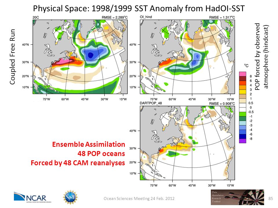
Coupled Free Run POP forced by observed atmosphere (hindcast) Ensemble Assimilation 48 POP oceans Forced by 48 CAM reanalyses Physical Space: 1998/1999 SST Anomaly from HadOI-SST 85Ocean Sciences Meeting 24 Feb. 2012
86
Example: cross section along Kuroshio; model separates too far north. 86 Challenges where ocean model is unable, or unwilling, to simulate reality. Ocean Sciences Meeting 24 Feb. 2012 Regarded to be accurate. Free run of POP, the warm water is too far North.

87
time = 10days time = 20days time = 30days time = 60daystime = 50days time = 40days 87 Initially warm water goes too far north. Many observations are rejected (red), but others (blue) move temperature gradient south. Adaptive inflation increases ensemble spread as assimilation struggles to push model towards obs. Latitude Temperature Challenges in correcting position of Kuroshio. 60-day assimilation starting from model climatology on 1 January 2004. Ocean Sciences Meeting 24 Feb. 2012
, but others (blue) move temperature gradient south. Adaptive inflation increases ensemble spread as assimilation struggles to push model towards obs. Latitude Temperature Challenges in correcting position of Kuroshio. 60-day assimilation starting from model climatology on 1 January Ocean Sciences Meeting 24 Feb")
88
time = 10days time = 20daystime = 30days 88 Observations keep pulling the warm water to the south; Model forecasts continue to quickly move warm water further north. Inflation continues to increase spread. Model forecasts finally fail due to numerical issues. Black dashes show original model state from 10 January. Challenges in correcting position of Kuroshio. 60-day assimilation starting from model climatology on 1 January 2004. time = 60daystime = 50days time = 40days Latitude Temperature Ocean Sciences Meeting 24 Feb. 2012 Green dashed line is posterior at previous time, Blue dashed line is prior at current time, Ensembles are thin lines.

89
time = 10days time = 20daystime = 30days time = 60daystime = 50days time = 40days 89 60-day assimilation starting from model climatology on 1 January 2004. Assimilation cannot force model to fit observations. Use of adaptive inflation leads to eventual model failure. Reduced adaptive inflation can lead to compromise between observations and model. Latitude Temperature Challenges in correcting position of Kuroshio. Ocean Sciences Meeting 24 Feb. 2012

90
Very certain that model predictions are different from observations. Very certain that small correlations have large errors. Moderately confident that large correlations are ‘realistic’. Very uncertain about state in sparse/unobserved regions. Must Calibrate and Validate results (adaptive inflation/localization). There may not be enough observations to do this many places. First order of business: Improving models. DA can help with this. Ensemble DA and UQ for Global Ocean Models 90
. There may not be enough observations to do this many places. First order of business: Improving models. DA can help with this. Ensemble DA and UQ for Global Ocean Models 90.")
91
Ocean Sciences Meeting 24 Feb. 2012 http://www.image.ucar.edu/DAReS/DART/ Code to implement all of the algorithms discussed are freely available from: 91

Similar presentations


 Rowan Sutton (Uni. Reading) and Doug Smith (UK Met Office) Analysis of a decadal prediction system:>")


>")


 experiments to quantify model errors.>")