1. Chapter 7: Stochastic Inventory Model Proportional Cost Models: x: initial inventory, y: inventory position (on hand + on order-backorder),  : random demand,  (  ),  (  ), (y-  ) + : ending inventory position, N.B.L, (y-  ) : ending inventory position, B.L,  =1/(1+r) : discount factor, ordering cost : c(y-x), holding cost : h (y-  ) + penalty cost : p(  -y) + salvage cost : -  s(y-  ) +

2. Minimum cost f(x) satisfies: L(y) convex, L’(  ) < -c (otherwise never order) L′ eventually becomes positive

3. Example c=$1, h=1¢ per month,  =0.99, p=$2(NBL), p=$0.25(BL), s=50 ¢, c+h-  s=51.5 ¢, NBL: p-c = 100 ¢, BL: p-c(1-  )=24 ¢,

4. Set up cost K L(x) if we order nothing K+c(S-x)+L(S) if we order upto S If we order, L’(S)+c=0. Use the cheaper of alternatives L(x) and K+ c(S-x)+L(S) Sx cost L(x) K K sSx L(x)+cx c s K+c(S-x)+L(S)

5. Two-bin or (s,S) policy order S-x if x ≤ s order nothing if x > s Multiperiod models Infinite Horizon (f 1000 & f 1001 cannot be different)

6. Taking derivative of {} If f convex, find S the base stock level, then for x ≤ S We see from (11) that f’(x)=-c for x ≤ S. (12)

7. Proportional costs: So that

8. Example 4:

9. Example 5:

10. Intuition: The current period would be a separate one period if we know what the next period would be willing to pay for our leftover inventory. Assuming we are not “overstocked”, every unit leftover will mean the next period will order one less, thus saving c. So the next period should be willing to pay c per unit in salvage for one leftover inventory.

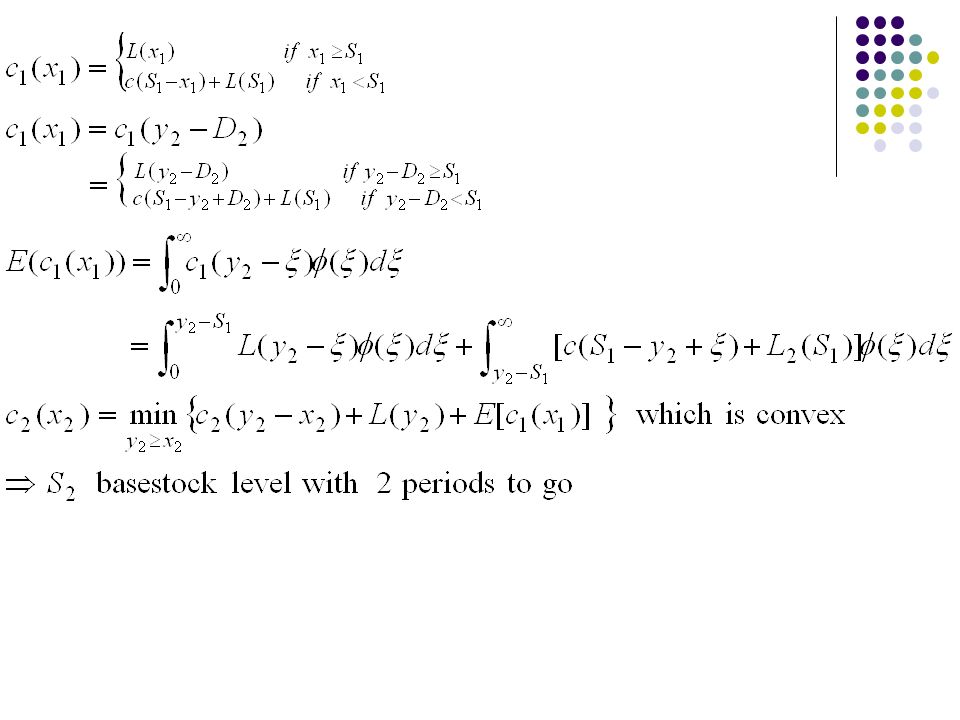
12. Multiperiod models: No Setup Cost Begin with two periods Demand D 1, D 2, i.i.d Density:  (  ) L(y) = expected one period holding+ shortage penalty cost; strictly convex with linear cost and  (  ) >0, c purchase cost /unit c 1 (x 1 ) optimal cost with 1 period to go; c+L’(S 1 )=0 while S 1 is the optimal base stock level.

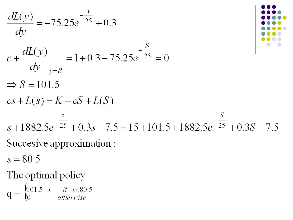
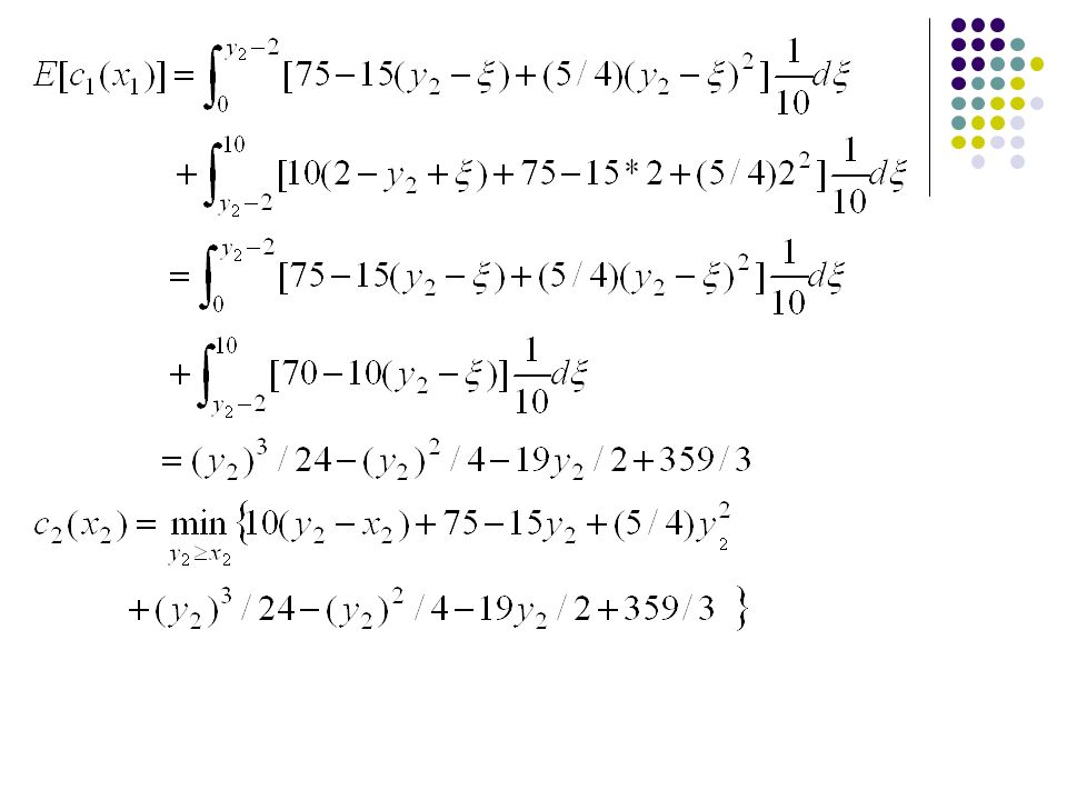
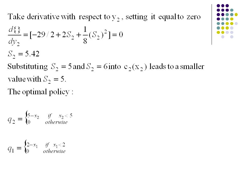
14. Example: c=10, h=10, p=15 the demand density is Solution:

17. Multi-Period Dynamic Inventory Model with no Setup Cost C n (x n ): n periods to go,  : discount factor. DP equations:

18. Multi-Period Dynamic Inventory Model with Setup Cost

19. Multi-Period Dynamic Inventory Model with Lead Times Lead time: