1. Air Pressure and Winds

4. Pressure Fluctuations Figure 9.3 Solar heating of ozone gasses in the upper atmosphere, and of water vapor in the lower atmosphere, can trigger oscillating thermal tides of sea-level pressure change.

5. Pressure Scale & Units Figure 9.4 Many scales are used to record atmospheric pressure, including inches of mercury (Hg) and millibars (mb). The National Weather Service uses mb, but will convert to metric units of hectopascals (hPa). The conversion is simply 1 hPa = 1 mb.

6. Pressure Measurement Changes in atmospheric pressure are detected by a change in elevation of a barometric fluid or change in diameter of an aneroid cell, which indicates changing weather. Average sea level pressure is 29.92 in Hg, or 1013.25 mb. Figure 9.5 Figure 9.6

7. Pressure Trends Figure 9.7 Barographs provide a plot of pressure with time, and are useful in weather analysis and forecasting. Altimeters convert pressure into elevation, and are useful in steep terrain navigation or flying. Both use aneroid cells.

8. Pressure Reading & Reporting Figure 9.8 Increase terrain elevation and decrease column of air above. To remove the effect of elevation, station pressure is readjusted to sea level pressure at ~10mb/100m. Isobars show geographic trends in pressure, and are spaced at 4 mb intervals.

9. Single-Cell Circulation Model Figure 11.1A The basis for average air flow around the earth can be examined using a non- rotating, non-tilted, ocean covered earth. Heating is more intense at the equator, which triggers Hadley cells to redistribute rising heat from the tropical low to the polar highs.

10. Ecclesiastes 1 6 The wind goeth toward the south, and turneth about unto the north; it whirleth about continually, and the wind returneth again according to his circuits.

13. ITCZ

16. ITCZ Limits

17. Three Cell Circulation Model A rotating earth breaks the single cell into three cells. The Hadley cell extends to the subtropics, the reverse flow Ferrel cell extends over the mid latitudes, and the Polar cell extends over the poles. The Coriolis force generates westerlies and NE trade winds, and the polar front redistributes cold air. Figure 11.2A

23. HURRICANE IVAN DISCUSSION NUMBER 44 NWS TPC/NATIONAL HURRICANE CENTER MIAMI FL 5 AM EDT MON SEP 13 2004 THE TRACK SCENARIO REMAINS THE SAME. THE HURRICANE IS FORECAST TO GRADUALLY TURN NORTHWARD OVER THE NEXT 72 HOURS INTO A WEAKNESS IN THE SUBTROPICAL RIDGE...AND THEN NORTHEASTWARD AS IT APPROACHES THE WESTERLIES.

24. 2002

25. Observed Winds in January Observed average global pressure and winds have increased complexity due to continents and the tilted earth. Differential ocean-land heating creates areas of semi- permanent high and low pressure that guide winds and redistribute heat. Figure 11.3A

26. Observed Winds in June Global pressure and wind dynamics shift as the Northern Hemisphere tilts toward the sun, bringing the inter-tropical convergence zone, the Pacific high, and blocking highs in the southern oceans northward. Figure 11.3B

27. North American Winter Weather Figure 11.4 Semi- permanent highs redirect North American winds, such as cold interior southerly flow from the Canadian high. The Polar front develops a wave like pattern as air flows around lows.

28. Global Precipitation Patterns Global low pressure zones around the equator and 60° latitude generate convergence at the surface, rising air and cloud formation. Zones of high pressure at 30° and the Poles experience convergence aloft with sinking, drying air. Figure 11.5

29. http://www.eoascientific.com/campus/earth/multimedia/coriolis/view_interactive

41. Coastal Summer Weather The semi-permanent Pacific high blocks moist maritime winds and rain from the California coast, while the Bermuda high pushes moist tropical air and humidity over the eastern states. Figure 11.6

42. Coastal Winter Weather During winter months, the Pacific high migrates southward and allows for maritime winds with moisture and rains to reach California. On the east coast, precipitation is rather even throughout the year. Figure 11.7

43. January Winds Aloft Land-sea temperature differences trigger ridges and troughs in the isobaric surface. Figure 11.8A

44. June Winds Aloft Horizontal temperature gradients establish pressure gradients that cause westerly winds in the mid latitudes. Figure 11.8B

46. Jet Stream Figure 11.9 High velocity Polar and subtropical jet stream winds are located in the lower tropopause, and they oscillate along planetary ridges and troughs. Figure 11.10

47. 300 mb Winds & Jets Figure 11.11 300 mb pressure surface maps illustrate lines of equal wind speed (isotachs) as the jets meander. Jet streaks are the maximum winds, exceeding 100 knots.

48. Polar Jet Formation Steep gradients of temperature change at the Polar front trigger steep pressure gradients, which then forces higher velocity geostrophic winds. This is the trigger for jet stream flow. Figure 11.13A

49. Winds & Angular Momentum Angular momentum is the product of mass, velocity, and the radius of curvature and it must be conserved. As northward- flowing air experiences a smaller radius, it increases in velocity and augments the jet stream flow. Figure 11.14

56. 14 September 04 http://www.wunderground.com/US/Region/US/JetStream.html http://www.wunderground.com/US/Region/US/JetStream.html

57. http://weather.unisys.com/upper_air/ua_500.html

65. Smoothed Isobar Maps Figure 9.9A Continental maps of station recorded sea-level pressure are often smoothed and simplified to ease interpretation. Smoothing adds error to those already introduced by error in instrument accuracy.

66. Constant Height Chart Maps of atmospheric pressure, whether at sea level or 3000 m above sea level, show variations in pressure at that elevation. Figure 9.10

67. Constant Pressure Chart Figure 9.11 Maps of constant pressure provide another means for viewing atmospheric dynamics. In this example, there is no variation in elevation for a pressure of 500 mb.

68. Variation in Height Isobaric (constant pressure) surfaces rise and fall in elevation with changes in air temperature and density. A low 500 mb height indicates denser air below, and less atmosphere and lower pressure above. Contour lines indicate rates of pressure change. Figure 9.12 Figure 9.13

69. Ridges & Troughs Upper level areas with high pressure are named ridges, and areas with low pressure are named troughs. These elongated changes in the pressure map appear as undulating waves. Figure 9.14

70. Surface & 500 mb Maps Surface maps chart pressure contours, highs and lows, and wind direction. Winds blow clockwise around highs, called anticyclones. 500 mb maps reveal patterns that on average are 5600 m above the surface, where westerly winds rise and fall across ridges and troughs. Figure 9.15A

71. Forces & Motion Pressure forces are only one influence on the movement of atmospheric air. Air responds similarly as water to this force, moving from higher pressure to lower pressure. Centripetal, friction, and apparent Coriolis are other forces, however, determining winds. Figure 9.16

72. Pressure Gradient Force Figure 9.17 Change in pressure per change in distance determines the magnitude of the pressure gradient force (PGF). Greater pressure changes across shorter distances creates a larger PGF to initiate movement of winds. Figure 9.18

73. PGF vs. Cyclonic Winds Pressure gradient force (PGF) winds acting alone would head directly into low pressure. Surface observations of winds, such as the cyclonic flow around this low, reveal that PGF winds are deflected by other forces. Figure 9.19

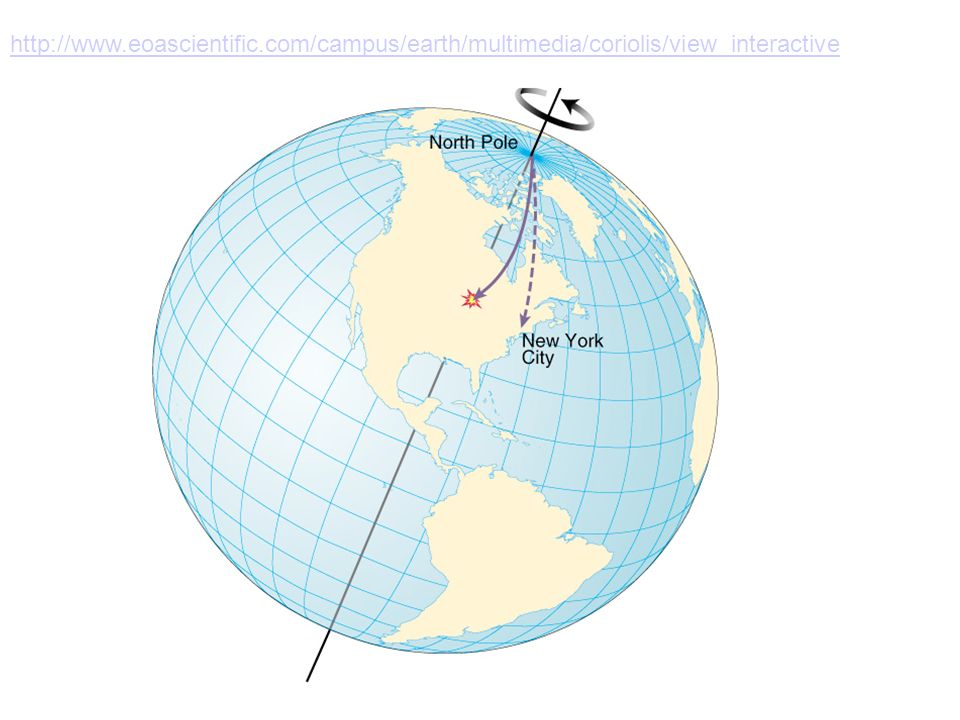
74. Apparent Coriolis Force Earth's rotation transforms straight line motion into curved motion for an outside viewer. The Coriolis force explains this apparent curvature of winds to the right due to rotation. Its magnitude increases with wind velocity and earth's latitude. Figure 9.20 Figure 9.21

75. Geostrophic Wind Figure 9.23 Winds have direction and magnitude, and can be depicted by vectors. Observed wind vectors are explained by balancing the pressure gradient force and apparent Coriolis force. These upper level geostrophic winds are parallel to pressure contours.

76. Wind Speed & Pressure Contours Just as a river speeds and slows when its banks narrow and expand, geostrophic winds blowing within pressure contours speed as contour intervals narrow, and slow as contour intervals widen. Figure 9.24

77. Isobars & Wind Prediction Figure 9.25A Upper level pressure maps, or isobars, enable prediction of upper level wind direction and speed.

78. Centripetal Acceleration & Cyclones Acceleration is defined by a change in wind direction or speed, and this occurs as winds circle around lows (cyclones) and highs (anticyclones). Centripetal force is the term for the net force directing wind toward the center of a low, and results from an imbalance between the pressure gradient and Coriolis forces. Figure 9.26A

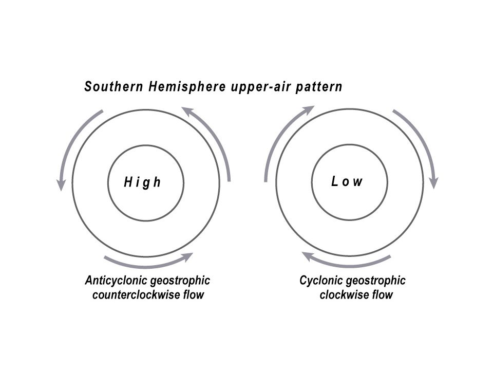
79. Northern & Southern Hemisphere Flow Figure 9.27A Winds blow counterclockwise around low pressure systems in the Northern Hemisphere, but clockwise around lows in the Southern Hemisphere.

80. Meridional & Zonal Flow Wind direction and speed are indicated by lines, barbs, and flags, and appear as an archer's arrow. Upper level winds that travel a north-south path are meridional, and those traveling a west-east path are zonal. Figure 9.28

81. Friction & Surface Winds Surface objects create frictional resistance to wind flow and slows the wind, diminishing the Coriolis force and enhancing the effect of pressure gradient forces. The result is surface winds that cross isobars, blowing out from highs, and in toward lows. Figure 9.29A

82. Surface Flow at Lows & Highs Southern Hemisphere flow paths are opposite in direction to Northern Hemisphere paths, but the same principles and forces apply. Figure 9.30 Figure 9.31

83. Sensing Highs & Lows The location of high and low pressure centers are estimated by detecting surface wind direction and noting pressure, Coriolis, and friction forces. This figure illustrates the procedure when standing aloft and at the surface. Figure 9.32A

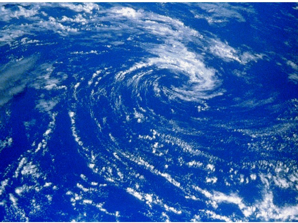
84. Vertical Air Motion Winds converging into a low pressure center generate upward winds that remove the accumulating air molecules. These updrafts may cause cloud formation. Likewise, diverging air molecules from a high pressure area are replenished by downward winds. Figure 9.33