Download presentation
Presentation is loading. Please wait.

1
Chapter Columns

2
10.1 Introduction Column = vertical prismatic members subjected to compressive forces Goals of this chapter: Study the stability of elastic columns Determine the critical load Pcr The effective length Secant formula

3
Previous chapters: -- concerning about (1) the strength and (2) excessive deformation (e.g. yielding) This chapter: -- concerning about (1) stability of the structure (e.g. bucking)
 stability of the structure (e.g. bucking)")
4
10.2 Stability of Structures
Concerns before: Stable? Unstable? New concern: (10.1) (10.2)
 (10.2)")
5
The system is unstable if
Since (10.2) The system is stable, if The system is unstable if A new equilibrium state may be established
 The system is stable, if. The system is unstable if. A new equilibrium state may be established.")
6
The new equilibrium position is:
(10.3) or
 or.")
7
After the load P is applied, there are three possibilities:
1. P < Pcr – equilibrium & = 0 -- stable 2. P > Pcr – equilibrium & = -- stable 3. P > Pcr – unstable – the structure collapses, = 90o

8
10.3 Euler’s Formula for Pin-Ended Columns
Determination of Pcr for the configuration in Fig ceases to be stable Assume it is a beam subjected to bending moment: (10.4) (10.5)
 (10.5)")
9
Defining: @ x = 0, y = 0 B = 0 @ x = L, y = 0
(10.6) (10.7) The general solution to this harmonic function is: (10.8) B.C.s: @ x = 0, y = B = 0 @ x = L, y = 0 Eq. (10.8) reduces to (10.9)
 (10.7) The general solution to this harmonic function is: (10.8) x = 0, y = 0 B = x = L, y = 0. Eq. (10.8) reduces to. (10.9)")
10
1. A = 0 y = 0 the column is straight!
(10.9) Therefore, 1. A = 0 y = 0 the column is straight! 2. sin pL = 0 pL = n p = n /L (10.6) Since We have (10.10) For n = 1 -- Euler’s formula (10.11)
 Therefore, 1. A = 0 y = 0 the column is straight! 2. sin pL = 0 pL = n p = n /L (10.6) Since. We have. (10.10) For n = Euler’s formula. (10.11)")
11
Substituting Eq. (10.11) into Eq. (10.6),
Therefore, Hence Equation (10.8) becomes (10.12) This is the elastic curve after the beam is buckled.
 becomes. (10.12) This is the elastic curve after the beam is buckled.")
12
1. A = 0 y = 0 the column is straight!
(10.9) 1. A = 0 y = 0 the column is straight! 2. sin pL = 0 pL = n If P < Pcr sin pL 0 Hence, A = 0 and y = 0 straight configuration
 1. A = 0 y = 0 the column is straight! 2. sin pL = 0 pL = n If P < Pcr sin pL 0. Hence, A = 0 and y = 0 straight configuration.")
13
L/r = Slenderness ratio
Critical Stress: Introducing Where r = radius of gyration Where r = radius of gyration (10.13) L/r = Slenderness ratio
 L/r = Slenderness ratio.")
14
10.4 Extension of Euler’s Formula to columns with Other End Conditions
Case A: One Fixed End, One Free End (10.11') (10.13') Le = 2L
 (10.13 ) Le = 2L.")
15
Hence, Le = L/2 Case B: Both Ends Fixed At Point C RCx = 0 Q = 0
Point D = inflection point M = 0 AD and DC are symmetric Hence, Le = L/2

16
M = -Py - Vx Case C: One Fixed End, One Pinned End Since Therefore,
The general solution: The particular solution:

17
into the particular solution, it follows
Substituting into the particular solution, it follows As a consequence, the complete solution is (10.16)
")
18
(10.16) B.C.s: @ x = 0, y = 0 B = 0 @ x = L, y = 0 (10.17) Eq. (10.16) now takes the new form
 now takes the new form.")
19
B.C.s: @ x = L, dy/dx = = 0 Taking derivative of the question,
(10.18) (10.17) (10.19)
 (10.17) (10.19)")
20
Le = 0.699L 0.7 L Solving Eq. (10.19) by trial and error, Since
Therefore, Solving for Le Case C Le = 0.699L 0.7 L

21
Summary

22
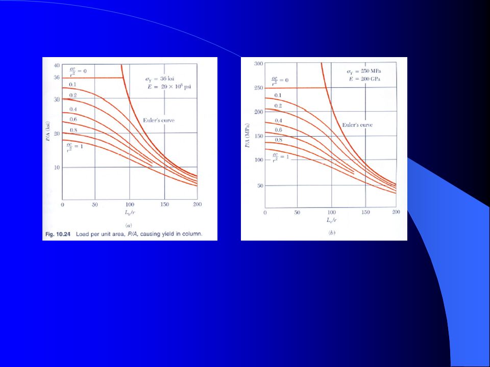
10.5* Eccentric Loading; the Scant Formula

23
Secant Formula: If Le/r << 1, Eq. (10.36) reduces to (10.36)
(10.37)
")
25
10.6 Design of Columns under a Centric Load

26
10.6 Design of Columns under a Centric Load
Assumptions in the preceding sections: -- A column is straight -- Load is applied at the center of the column -- < y Reality: may violate these assumptions -- use empirical equations and rely lab data

27
Test Data: Facts: 1. Long Columns: obey Euler’s Equation
2. Short Columns: dominated by y 3. Intermediate Columns: mixed behavior

28
Empirical Formulas:

29
Real Case Design using Empirical Equations:
1. Allowable Stress Design Two Approaches: 2. Load & Resistance Factor Design

30
Structural Steel – Allowable Stress Design
Approach I -- w/o Considering F.S. 1. For L/r Cc [long columns]: [Euler’s eq.] 2. For L/r Cc [short & interm. columns]: where

31
Approach II -- Considering F.S.
1. L/r Cc : (10.43) 2. L/r Cc : (10.45)
 2. L/r Cc : (10.45)")
32
10.7 Design of Columns under an Eccentric Load
(10.56) 1. The section is far from the ends 2. < y (10.57) Two Approaches: (I) Allowable Stress Method (II) Interaction Method
 1. The section is far from the ends. 2. < y. (10.57) Two Approaches: (I) Allowable Stress Method. (II) Interaction Method.")
33
I. Allowable-Stress Method
(10.58) -- all is obtained from Section 10.6. -- The results may be too conservative.
 -- all is obtained from Section The results may be too conservative.")
34
II. Interaction Method Case A: If P is applied in a plane of symmetry:
(10.59) (Interaction Formula) (10.60) -- determined using the largest Le
 (Interaction Formula) (10.60) -- determined using the largest Le.")
35
Case B: If P is NOT Applied in a Plane of Symmetry:
(10.61)
")
Similar presentations


 MAE 316 – Strength of Mechanical Components>")
 (How to find k?)>")

 Compression Members Columns: Beam-Columns: Columns Theory:>")

