1. Dr. Z. R. Ghassabi z.r.ghassabi@gmail.com Tehran shomal University Spring 2015 z.r.ghassabi@gmail.com Digital Image Processing Session 3 1

2. Outline Introduction Digital Image Fundamentals Intensity Transformations and Spatial Filtering Filtering in the Frequency Domain Image Restoration and Reconstruction Color Image Processing Wavelets and Multi resolution Processing Image Compression Morphological Operation Object representation Object recognition 2

3. Outline of Chapter 3 Basic Intensity Transformation Functions Negative, Log, Gamma Piecewise-Linear Transformation Functions Contrast stretching, contrast slicing, bit-plane slicing Histogram Processing Histogram Stretching, Histogram Shrink, Histogram Sliding, Histogram equalization, adaptive local histogram, histogram matching, local histogram equalization, histogram statistics Fundamentals of Spatial Filtering Smoothing Spatial Filters, Sharpening Spatial Filters, Combining Spatial Enhancement Tools

4. Image Enhancement Methods – Spatial Domain: Linear Nonlinear – Frequency Domain: Linear Nonlinear

5. Image Enhancement Spatial Domain

6. Image Enhancement Example: Image Subtraction for enhancing Differences

7. Image Enhancement Frequency Domain

8. Image Transforms

9. Image Enhancement in spatial Domain (Transformation) For 1  1 neighborhood: – Contrast Enhancement/Stretching/Point process For w  w neighborhood: – Filtering/Mask/Kernel/Window/Template Processing

10. Image Enhancement in spatial Domain Input gray level, r Output gray level, s Negative Log nth root Identity nth power Inverse Log Some Basic Intensity Transformation Functions

11. Image Negatives Image Negatives: L x 0 L y y=L-x

12. Image Negatives

13. Log Transformation

14. c=100 L x 0 y

15. Log Transformation Range Compression

16. Power-Law(Gamma) Transformations

17. Gamma Correction:

18. Power-Law(Gamma) Transformations (Effect of decreasing gamma)

19. Power-Law(Gamma) Transformations (Effect of increasing gamma)

20. Power-Law(Gamma) Transformations Medical Example

21. Piecewise-Linear Transformation Functions Contrast Stretching Contrast slicing Bite-Plane slicing

22. Contrast Stretching L x 0 ab yaya ybyb y

23. Contrast stretching Original C. S. THR.

24. Contrast Stretching

25. L x 0ab y Clipping:

26. MATLAB Tutorial imadjust(I, [low-in, high-in],[low-out, high-out]) low-in high-in low-out high-out Output Image Input Image

27. مناسب ترین مقدار چیست؟ MATLAB Tutorial imadjust(I, [low-in, high-in],[low-out, high-out], gamma) imadjust(I, [0.1, 0.7],[0, 1], gamma) low-in high-in low-out high-out Output Image Input Image

28. MATLAB Tutorial Use Min and Max gray-levels – Low-in: Double(min(I(:))/255) – max-in: Double(max(I(:))/255) Use stretchlim(I) imadjust(I,stretchlim(I),[low-out, high-out], gamma)

29. MATLAB Tutorial low-in high-in low-out high-out Output Image Input Image

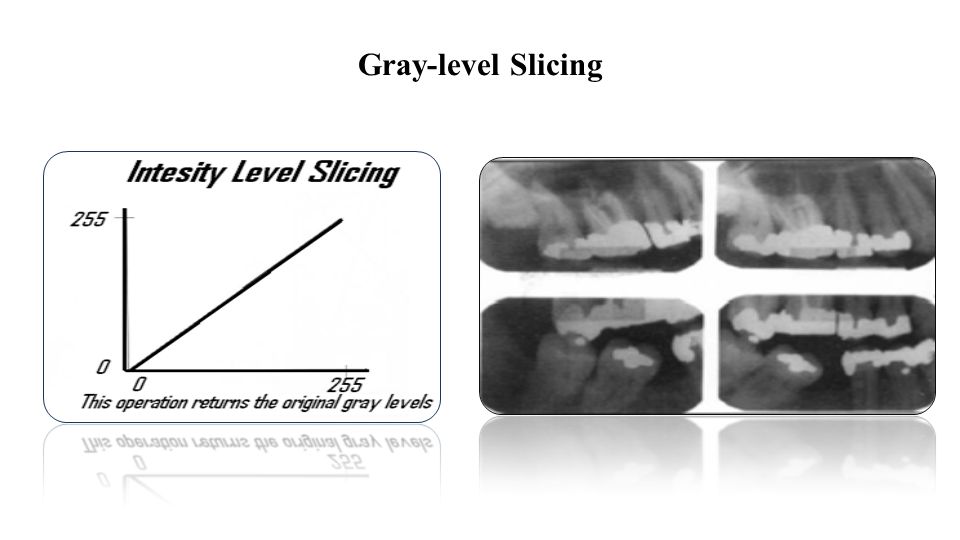
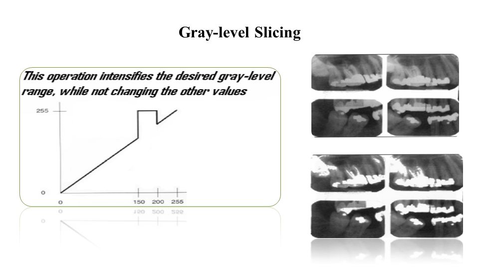
30. Gray-level Slicing

31. Gray-level Slicing

34. Gray-level Slicing

35. Bit-plane Slicing Highlighting the contribution made to total image appearance by specific bits Suppose each pixel is represented by 8 bits Higher-order bits contain the majority of the visually significant data Useful for analyzing the relative importance played by each bit of the image

36. Bit-plane Slicing

37. The (binary) image for bit-plane 7 can be obtained by processing the input image with a thresholding gray-level transformation. Map all levels between 0 and 127 to 0 Map all levels between 129 and 255 to 255

38. Bit-plane Slicing Fractal Image

39. Bit-plane 7Bit-plane 6 Bit-plane 5Bit-plane 4Bit-plane 3 Bit-plane 2Bit-plane 1Bit-plane 0

40. Bit-plane Slicing

41. Histogram Processing Enhancement based on statistical Properties: Local, Global Histogram Definition h(r k )=n k Where r k is the kth gray level and n k is the number of pixels in the image having gray level r k Normalized histogram: P(r k )=n k /n Histogram of an image represents the relative frequency of occurrence of various gray levels in the image

42. Histogram Example

43. MATLAB Tutorial Hist(double(I(:)),50) imhist(I)

44. Histogram Examples Histogram Visual Meaning: – Dark – Bright – Low Contrast – High Contrast

45. Histogram Modification Histogram Stretching Histogram Shrink Histogram Sliding

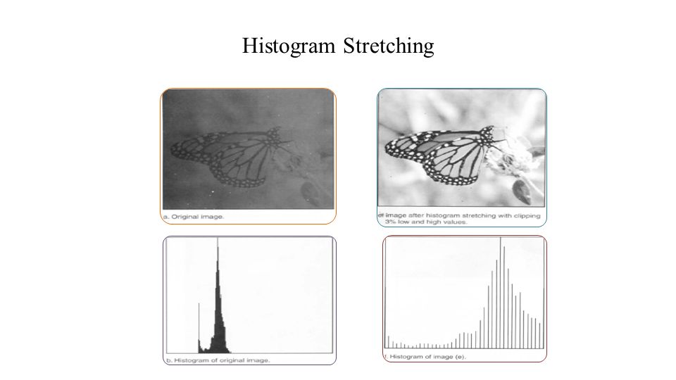
46. Histogram Stretching

49. Histogram Shrinking

50. Histogram Shrinking

51. Histogram Sliding

52. Histogram Equalization PDF تناظر بین x و U اکیدا صعودی بودن CDF هست. برای اکیدا صعودی بودن تابع CDF باید مشتق آن یعنی PDF همیشه بزرگتر از صفر باشد. F: X-------->[0,1] U=F(X) چون تابع یک به یک هست پس معکوس هم دارد. X=F -1 (U) x 1 0 CDF U متغیر تصادفی

53. Histogram Equalization

54. توزیع آماری u مستقل از مقدار x و همیشه یکنواخت بین 0 و یک هست. u~U(0,1) X های ورودی را بین 0 و یک توزیع میکند. هیستوگرام U

55. Histogram Equalization r 1 0 CDF S=T(r) PDF PrPr سطح زیر منحنی S~U(0,1) هیستوگرام U هیستوگرام تصویر ورودی روشنایی تصویر ورودی r

56. Histogram Equalization r 1 0 CDF S=T(r) PDF PrPr روشنایی تصویر ورودی r هیستوگرام تصویر ورودی

57. Histogram Equalization

58. Histogram Equalization

59. MATLAB Tutorial histeq(I)

60. Histogram Equalization

61. Adaptive Contrast Enhancement (ACE)

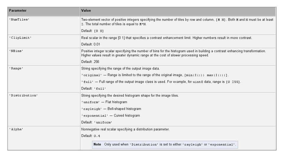
64. MATLAB Tutorial I2=adapthisteq( I,'clipLimit',0.015,'Distribution','rayleigh'); clear all; close all; clc; [f1, pp1] = uigetfile('*.jpg', 'Pick a image'); I1Name = sprintf('%s%s',pp1,f1); I=imread(I1Name); if ndims(I)==3 I1=rgb2gray(I); end I2=adapthisteq( I1,'clipLimit',0.015,'Distribution','rayleigh'); figure(); subplot(1,2,1); imshow(I1); subplot(1,2,2); imshow(I2);

66. Adaptive Histogram Equalization

67. Histogram Matching prpr pzpz Histeq(I,hgram)

68. Histogram matching: Obtain the histogram of the given image, s=T(r) Precompute a mapped level S k for each level r k Obtain the transformation function G from the given p z (z) Precompute Z k for each value of r k Map r k to its corresponding level S k ; then map level S k into the final level Z k Histogram Matching r S 0 CDF S=T(r) PDF PrPr r هیستوگرام تصویر ورودی 0 pzpz هیستوگرام دلخواه

69. Histogram Matching (Specification) برای یک تصویر 64*64 هیستوگرام طوری تبدیل شود که دارای مقادیر مشخص شده در شکل b باشد.

70. Histogram Matching (Specification) S 0 =1, G(z 3 )=1, s 0 --- >z 3 هر پیکسلی که مقدارش در تصویر تعدیل هیستوگرام یک هست به مقداری برابر سه در هیستوگرام مشخص شده نگاشت می شود.

71. Image is dominated by large, dark areas, resulting in a histogram characterized by a large concentration of pixels in pixels in the dark end of the gray scale Histogram Matching (Specification)

72. Notice that the output histogram’s low end has shifted right toward the lighter region of the gray scale as desired. Histogram Matching (Specification)

73. Desired Initial CDF Modified CDF Histogram Matching (Specification)

74. Local Histogram Processing a)Original image b)global histogram equalization c)local histogram equalization using 7x7 neighborhood.

75. Histogram using a local 3*3 neighborhood Local Histogram Processing

76. Use of histogram statistics for image enhancement: r denotes a discrete random variable P(r i ) denotes the normalized histogram component corresponding to the i th value of r Mean: The n th moment: The second moment: Using Histogram Statistics

77. Global enhancement: The global mean and variance are measured over an entire image Local enhancement: The local mean and variance are used as the basis for making changes Using Histogram Statistics r s,t is the gray level at coordinates (s,t) in the neighborhood P(r s,t ) is the neighborhood normalized histogram component mean: local variance:

78. Mapping: E,K 0,K 1,K 2 are specified parameters M G is the global mean D G is the global standard deviation Using Histogram Statistics

79. A SEM sample images: Using Histogram Statistics

80. Local Mean Local Var E or one Using Histogram Statistics

81. Enhanced Images: Using Histogram Statistics

82. Fundamental of Spatial Filtering

83. The Mechanics of Spatial Filtering: -a +a -b+b Image size: M×N, x= 0,1,2,…,M-1 and y= 0,1,2,…,N-1 Mask size: m×n, a=(m-1)/2 and b=(n-1)/2 Correlation

84. Fundamental of Spatial Filtering

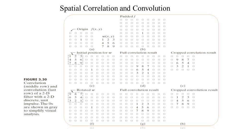
85. Spatial Correlation and Convolution

87. Vector Representation of Linear Filtering

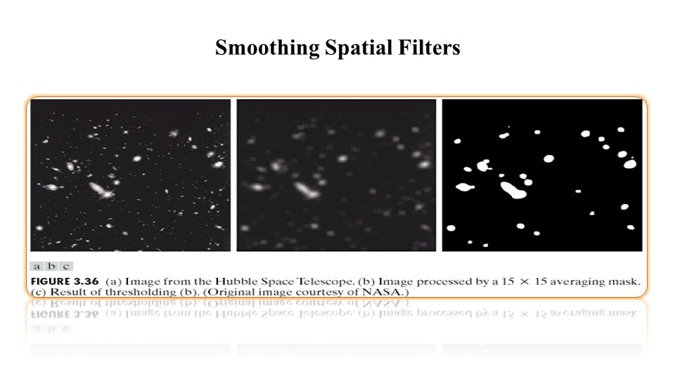
88. Smoothing Linear Filters : Noise reduction Smoothing of false contours Reduction of irrelevant detail Smoothing Spatial Filters

89. Image smoothing with masks of various sizes.

91. MATLAB Tutorial W=repmat(1/9,3,3); W=1/9*ones(3,3); a=2; W=ones(2*a+1) W=W/sum(W(:)); Img1=imread(‘image1.jpg’); Img2=imfilter(Img1,W);

92. MATLAB Tutorial Img2=imfilter(Img1,W,’symmetric’);

93. Order-statistic filters: Max Min Median filter: Replace the value of a pixel by the median of the gray levels in the neighborhood of that pixel  Noise-reduction Order-Static (Nonlinear) Filters

94. Median Filter

95. The first-order derivative: The second-order derivative Sharpening Spatial Filters Zero in flat region Non-zero at start of step/ramp region Non-zero along ramp Zero in flat region Non-zero at start/end of step/ramp region Zero along ramp

96. Sharpening Spatial Filters

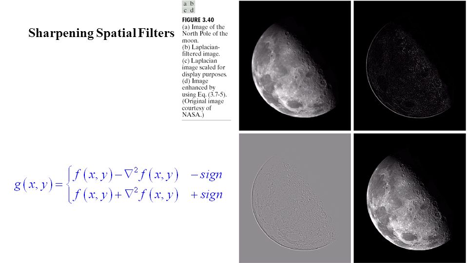
98. Use of second derivatives for enhancement-The Laplacian: Development of the method Sharpening Spatial Filters

99. Practically use:

100. Sharpening Spatial Filters

102. Two L. Mask SEM image a. Mask Result b. Mask Result (Sharper)

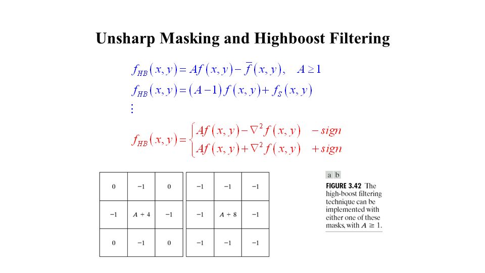
103. Unsharp masking Subtract a blurred version of an image from the image itself f(x,y) : The image, f ̄ (x,y): The blurred image High boost Filtering: Unsharp Masking and Highboost Filtering

106. Original Laplacian (A=0) Laplacian (A=1) Laplacian (A=1.7) Unsharp Masking and Highboost Filtering

107. Using first-order derivatives for (nonlinear) image sharpening, The gradient: The gradient: The magnitude is rotation invariant (isotropic) Using First-Order Derivative for (Nonlinear) Image Sharpening - The Gradient

108. Roberts Cross Gradient Sobel (2  1 for prewitt) and

109. Using the Gradient for Image Sharpening Sobel Gradient

110. Bone Scan Laplacian Original +Laplacian Soble of Original Combining Spatial Enhancement Tools

111. Smoothed Sobel (Orig. + L.)*S.Sobel Orig.+ (Orig. + L.)*S.Sobel Apply Power-Law Combining Spatial Enhancement Tools

112. Img0=im2double(img0); w=fspecial(type, parameters) W=fspecial(‘disk’,3); W=fspecial(‘gaussian’,101,10); W=fspecial(‘laplacian’,0); W=fspecial(‘log’,10,1); Img1=imfilter(Img0,W); figure();imshow(normalize(Img1)); C=-1; figure();imshow(img0+C*Img1); Wp=fspecial(‘prewitt’); Ws=fspecial(‘prewitt’); Img1=imfilter(Img0,Wp); Img2=imfilter(Img0,Ws); W=0.3*Wp+0.7*Ws; Img1=imfilter(Img0,W); Img1=imfilter(Img0,Wp); Img2=imfilter(Img0,Wp’); Imshow(sqrt(Img1.^2+Img2.^2) MATLAB Tutorial

113. function XN=Normalize(X) Xmin=min(X(:)); Xmax=max(X(:)); XN=((X-Xmin)/(Xmax-Xmin)).^beta; end MATLAB Tutorial

114. Img0=im2double(imread(‘….’)); M=3;N=5; Domain=ones(M,N); Img1=ordfilt2(img0,M*N, Domain); Img2=ordfilt2(img0,0, Domain); Img3=ordfilt2(img0,(M+N+1)/2, Domain); figure(); subplot(1,3,1); imshow(Img1); subplot(1,3,2); imshow(Img2); subplot(1,3,3); imshow(Img3); MATLAB Tutorial

115. Img0=im2double(imread(‘….’)); M=3;N=5; Domain=ones(M,N); Img1=imnoise(img0,’salt & pepper’); Img2=ordfilt2(img1,(M+N+1)/2, Domain); Img3=medfilt2(img1,[M N]); figure(); subplot(2,2,1); imshow(Img0); subplot(2,2,2); imshow(Img1); subplot(2,2,3); imshow(Img2); subplot(2,2,3); imshow(Img3); MATLAB Tutorial

116. MATLAB Command: – Image Statistics: means2, std2, corr2, imhist, regionprops – Image Intensity Adjustment: imadjust, histeq, adapthisteq, imnoise – Linear Filter: imfilter, fspecial, conv2, corr2, – Nonlinear filter: medfilt2, ordfilt2,

117. MATLAB Tutorial

118. End of Session 3