Download presentation
Presentation is loading. Please wait.

1
Calculus 1D With Raj, Judy & Robert

2
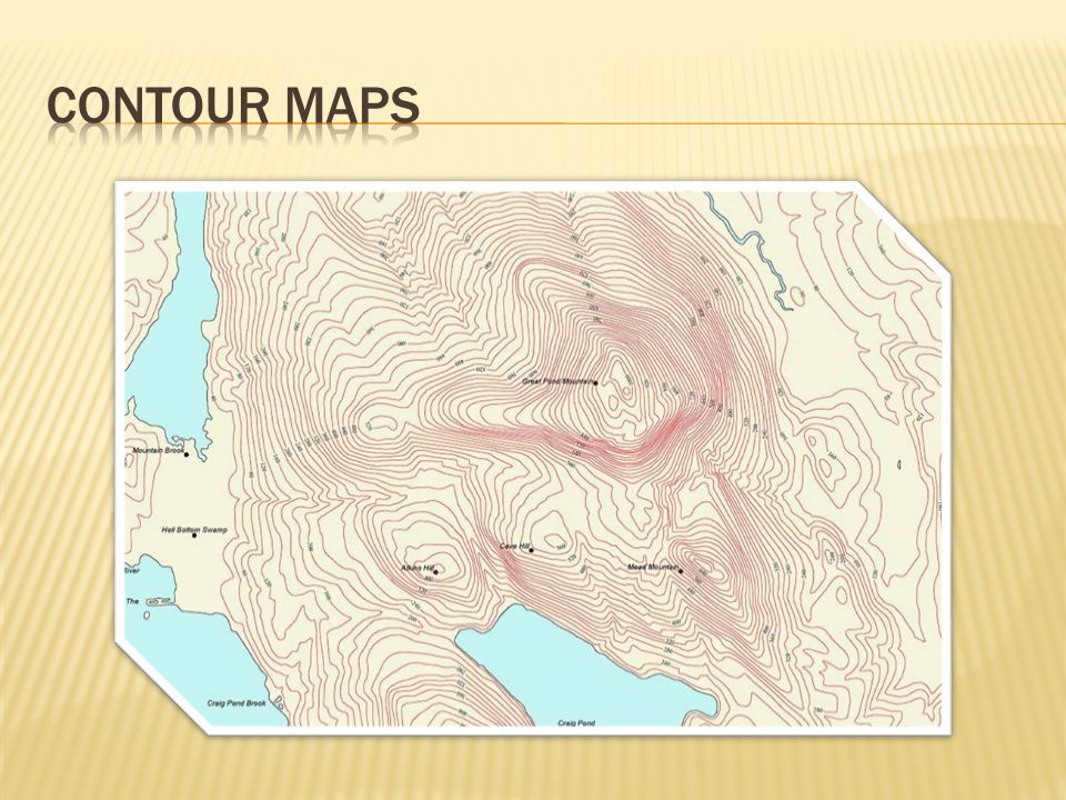
Hyperbolic & Inverse Contour Maps Vectors Curvaturez, Normal, Tangential Parameterization Coordinate Systems Taylor Expanzion Approximation Projectile Motion Keplers Laws of planetary motion Vector Fields Conservative Line Integrals Works Curl & Divergence Greens Theorem Stokes Theorem Surface Integration Divergence Theorem Maxwell’s Equations

4
Construction of bridges Hanging Cables or chains Secondary Mirrors in Telescopes Planetary Orbits Field Deflection

7
Restate a function in order to simplify its integration or derivation t is often used, but it is just a variable name This process simplifies integration of line integrals Parabolic Cylindrical Spherical

8
What are Taylor Series Used for? Limit of a Taylor Polynomial Uses multiple derivatives in order to find an estimation at a nearby point. More terms = better approx. Let f be a function with derivatives of order k for k=1,2,…,N in some interval containing a as an interior point. For any integer n from 0 through N The taylor polynomial of order n generated by f as x=a is the polynomial…

9
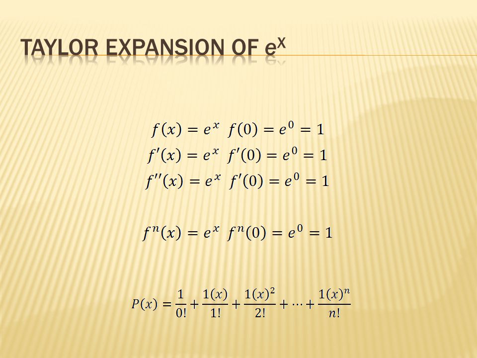
Estimate the value of e x at 0.05 What do we have? a = 0 f(x)=e x f’(x)=e x Start with the derivatives at that point
=e x f’(x)=e x Start with the derivatives at that point.")
11
Adding terms to the taylor expansion leads to greater convergence onto the function How did you think your calculator worked? See Freddies multiple variable discussion

12
Magnitude Direction Scalar Multiplication Scaled Vector V = 4V = Dot Product Scalar Value |V||U|Cos( ß) VU = (Vx*Ux)+(Vy*Uy)+(Vz*Uz) Cross Product Orthogonal Vector |V||U|Sin( ß) VXU = Common Arithmetic Operations
 VU = (Vx*Ux)+(Vy*Uy)+(Vz*Uz) Cross Product Orthogonal Vector |V||U|Sin( ß) VXU = Common Arithmetic Operations")
13
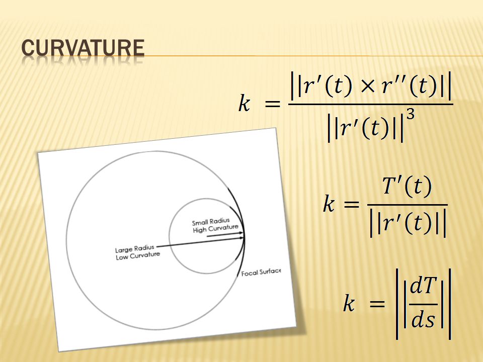
Unit Tangent Binormal (Will be a unit vector) Unit Normal direction
 Unit Normal direction")
15
Defined by a Vector Function, as a function of each component Curl & Divergence Flow Patterns Gradient

16
Smooth Check is a matrix of all variables and their partials We are effectively equating our vector field to the gradient of our function Path Independence Convert to polar No Singularities Magnetism Gravity Work Done

17
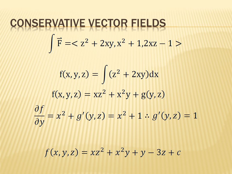
Smooth Check Check the partial derivatives Integrate One Component Constant function of others Partial with respect to another component y in this example Compare it to the y component and solve for g’(y,z) Repeat these two steps for the remaining components A conservative vector field has a constant in the very end, relating it to no other variables
 Repeat these two steps for the remaining components A conservative vector field has a constant in the very end, relating it to no other variables")
18
N/A 22 2 0 20

21
Curl is the tendency to rotate Divergence is the tendency to explode

22
The integral of the derivative over a region R is equal to the value of the function at the boundary B. Divergence Theorem R = Volume B = Surface Curl/Stokes Theorem R = Surface B = Line Integral

23
Integrate to see how a field acts upon a particle moving along a curve. Calculating the work done by a force that changes with time over a curve that changes with time Estimating wire weight, given a density function

24
Green is a simplification of Stokes, for 2D Simple Jordan Curve

25
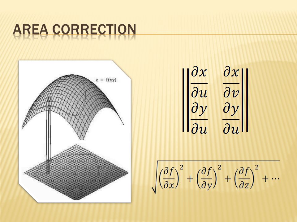
Flux aka Surface Integration Area Correction

26
Fluids into an area Based on volume changes CategoriesCategories: Structure of the Earth | Obsolete scientific theoriesStructure of the EarthObsolete scientific theories

27
1. The orbit of every planet is an ellipse with the sun at a focus 2. A line joining a planet and the sun sweeps out equal areas during equal intervals of time 3. The square of the orbital period of a planet is directly proportional to the cube of the semi-major axis of its orbit

28
Originally a radical claim, because the belief was that planets orbited in perfect circles. Ellipse for inner planets has such low eccentricity, so they can be mistaken for circles The orbit of every planet is an ellipse with the sun at a focus (r, theta) are heliocentric polar coordinates, p is the semi-latus rectum, and E is the eccentricity
 are heliocentric polar coordinates, p is the semi-latus rectum, and E is the eccentricity.")
29
Planets move faster the closer it is to the sun In a certain interval of time, the planet will travel from A to B In an equal interval of time, the planet will travel from C to D The resulting "triangles" have the same area Conservation of angular momentum A line joining a planet and the sun sweeps out equal areas during equal intervals of time

30
Is a way to compare the distances traveled between planets and how fast two planets travel, given the difference between the linear distances from the sun. Example: Say Planet R is 4 times as far from the sun as Planet B. So R must travel 4 times as far per orbit as B. R also travels at half the speed of B, so it will take R 8 times as long to complete an orbit as B. 3) "The square of the orbital period of a planet is directly proportional to the cube of the semi-major axis of its orbit." P is the orbital period of the planet and a is the semimajor axis of the orbit Formerly known as the harmonic law
 The square of the orbital period of a planet is directly proportional to the cube of the semi-major axis of its orbit. P is the orbital period of the planet and a is the semimajor axis of the orbit Formerly known as the harmonic law.")
31
Implications Time Dilation Relativity of simultaneity Composition of velocities Lorentz Contraction Inertia and Momentum Cassini Space Probe & Relativity © nasa.gov

32
http://blog.gneu.org bob.chatman@gmail.com

Similar presentations


 Universal Gravitation & SHM>")
 Universal Gravitation & SHM.>")

>")
 Enrichment Programme for Physics Talent 2006/07 Module I.>")


