1. Chapter 1 Vector analysis
August 22 Elementary approach
1. 1 Definitions, elementary approach
Scalar quantities: Quantities having magnitude only.
Length, mass, time, temperature, energy.
Vector quantities: Quantities having both magnitude and directions.
Displacement, velocity, acceleration, momentum, angular momentum, electric field, magnetic field, dipoles.
Tensor quantities: (Tensors of rank n) moment of inertia, electric permittivity, nonlinear susceptibility .
Geometrical representation of a vector:
An arrow.
Addition and subtraction:
Vector addition is commutative and associative.

2. Algebraic representation of a vector:
component, projection
direction cosine
unit vector, basis
more preferred form
most convenient for doing algebra
magnitude (length, norm)

3. 1. 2 Rotation of the coordinate axesV
scalar product (more later)
Kronecker delta symbol
Einstein’s summation convention: Any repeated indices are summed over, unless otherwise specified. Greatly simplifies many expressions.
Rotation matrix aij represents the transformation between the two sets of coordinates. Its elements are the projections between the two sets of bases.
Orthogonality conditions:
aij
Orthonormal
transformation

4. Components of a vector after transformation:
Question: Is electric current (I) a vector?
Redefinition of a vector quantity:
A quantity is a vector if its components transform as under an orthonormal transformation specified by aij.
For tensors:
Generalization of vectors. Vectors can also be
Complex quantities.
Functions.
Multi-dimensions or infinite dimensions.

5. Read: Chapter 1: 1-2
Homework: 1.1.1, 1.2.1(a)
Due: September 2

6. August 24,26 Scalar and vector products 1. 3 Scalar or dot productB A q
Geometric definition:
Scalar product is commutative and distributive.
Algebraic definition:
( , orthonormal)
Invariance of the scalar product under an orthogonal transformation:
We thus proved that A·B is indeed a scalar.

7. 1. 4 Vector or cross productB A q C
Geometric definition:
Meaning: area of the parallelogram formed by A and B.
Cross product is anticommutative:
Algebraic definition:
Levi-Civita symbol (antisymmetric tensor) eijk: 1 2 3 + -
Look at your watch.

8. Cross product is based on the nature of our 3-dimentional space.
Cross product in determinant form:
Cross product is based on the nature of our 3-dimentional space.
Matrix representation of cross product:
Example:

9. = the volume enclosed by the parallelepiped defined by A, B and C.
1. 5 Triple scalar product, triple vector product
Triple scalar product :
= the volume enclosed by the parallelepiped defined by A, B and C.

10. Can be proved by brute force (though not trivial).
Triple cross product :
Can be proved by brute force (though not trivial). C B q
B×C A
The “bac-cab” rule.

11. Read: Chapter 1: 3-5
Homework: 1.3.3, 1.4.7,1.5.12
Due: September 2

12. Reading: Proof that C=A×B is a vector:

13. About matrices:
Inverse matrix A-1 :
Transpose matrix Ã:
For orthonormal matrices:
About determinates:
Minor Mij: removing the ith row and the jth column
Cofactor Cij : (-1)i+j Mij
Expansion of a determinant:
Calculation of A-1:
For orthonormal matrices with |A|=1:

14. August 29, 31 Gradient, divergence and curl 1. 6 Gradient, 
Definition: In a 3D Cartesian coordinate system,
Example:
Central force:
Proof that j is a vector:

15. Geometrical interpretations:1)
The function j has the steepest change along the direction of its gradient. 2)
j is perpendicular to the surface of

16. 1. 7 Divergence ,· Definition: In a 3D Cartesian coordinate system,
Examples:
Physical meaning:
is the net outflow flux of j per unit volume.
B is solenoidal if

17. 1. 8 Curl,  Definition: In a 3D Cartesian coordinate system,
Example:
Physical meaning:
Set the coordinate system so that z is along at an arbitrarily chosen point. Suppose the coordinates of that point is then (x0, y0, z0 ).
is the total circulation of V per unit area.
V is irrotational if

18. 1. 9 Successive applications of 
Example: 1)
1. 9 Successive applications of  2) 3) 4)

19. More about Laplacian:

20. Reading: Physical meaning of Laplacian:
Laplacian measures the difference between the average value of the field around a point and the value of the field at that point.
If then j cannot increase or decrease in all directions.

21. Read: Chapter 1: 6-9
Homework: 1.6.3,1.6.4,1.7.5,1.8.4,1.8.11,1.8.13,1.8.14,1.9.7
Due: September 9

22. September 2,7 Gauss’ theorem and Stokes’ theorem
1. 10 Vector integration A B
Line integral:
Circulation:
(mostly used line integral)
If , the line integral is independent of the path between A and B:
The circulation of F around any loop is then 0:
Surface integral:
(mostly used surface integral, flux)
Volume integral:

23. Integral definition of gradient, divergence and curl:z dy dz y x dx
Proof: let

24. 1. 11 Gauss’ theorem Gauss’ theorem :
(Over a simply connected region.)
Proof: For a differential cube,
Sum over all differential cubes, at all interior surfaces will cancel, only the contributions from the exterior surfaces remain.

25. then use Gauss’ theorem.
Green’ theorem :
Proof:
then use Gauss’ theorem.
Variant:
Alternate forms of Gauss’ theorem :
These can also be obtained from the integral definition of gradient, divergence and curl.
Example of Gauss’ theorem: Gauss’ law of electric field

26. 1. 12 Stokes’ theorem Stokes’ theorem :
(Over a simply connected region. The surface does not need to be flat.)
Proof: Set the coordinate system so that x is along ds at an arbitrarily chosen point on the surface. Suppose the coordinates of that point is then (x0, y0, z0 ).
Sum over all differential squares, at all interior lines will cancel, only the contributions from the exterior lines remain.

27. Alternate forms of Stokes’ theorem :
Example of Stokes’ theorem: Faraday’s induction law
Stokes’ theorem for a curve on the x-y plane: Green’s theorem

28. Read: Chapter 1: 10-12
Homework: ,1.11.2,1.11.6,1.12.3,
Due: September 9

29. September 9 Gauss’ law and Dirac delta function 1. 14 Gauss’s law
Electric field of a point charge: q S S′
Gauss’ law:
Proof:
1) If S does not include q, using Gauss’ theorem,

30. 2) If S includes q, construct a small sphere S' with radius d around the charge and a small hole connecting S and S’. q S S′
If S includes multiple charges,
For a charge distribution,
Using Gauss’ theorem,

31. 1. 15 Dirac delta function Dirac delta function is defined such that
Especially,
Example:
Using the Dirac delta function,

32. Dirac delta function (distribution) is the limit of a sequence of functions, such as
The sequence of integrals has a limit:
We write it as implying that we are always doing the limit.

33. Properties of d (x):
Proof:

34. Read: Chapter 1: 13-15
Homework: ,1.13.9,1.14.3,1.15.7
Due: September 16

35. September 12 Helmholtz’s theorem 1. 16 Helmholtz’s theorem
The uniqueness theorem : A vector is uniquely specified within a simply connected region by given its 1) divergence , 2) curl, and 3) normal component on the boundary.
Proof:

36. Corollary: The solution of Laplacian equation is unique at a given boundary condition.

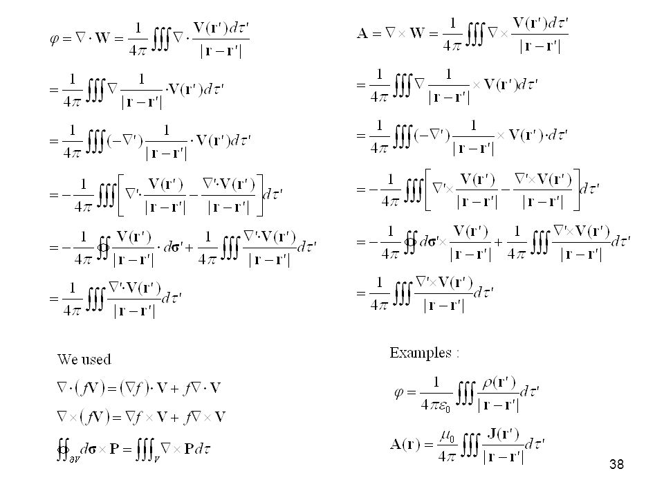
37. Helmholtz’s theorem (the fundamental theorem of vector calculus): Any rapidly decaying vector field (faster than 1/r at infinity) can be resolved into the sum of an irrotational vector field and a solenoidal vector field.
Proof: Let us prove that any vector V can be decomposed as
The explicit expressions of j and A are given later.

39. Read: Chapter 1: 16
Homework:
Due: September 23