Download presentation
Presentation is loading. Please wait.

1
Variational data assimilation in geomagnetism: progress and perspectives Andy Jackson, Kuan Li ETH Zurich & Phil Livermore University of Leeds

2
Outline Rationale for 4DVar Proof of concept: Hall effect dynamo (Hardcore Bayes: a prior pdf for core surface field estimation)
")
5
Convergence Degrees of freedom ->

6
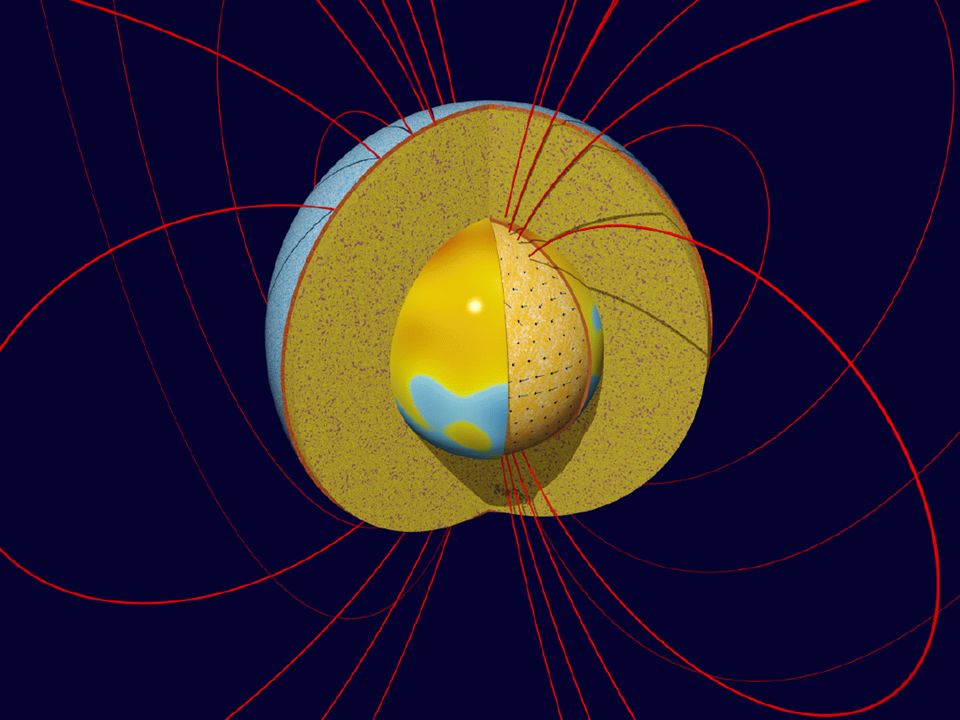
Visible and hidden parts of the magnetic field Based only on poloidal magnetic field data on the boundary of the core, can we infer interior properties (including those of the toroidal field)? Measurements

7
Technology transfer from meteorology: 4DVar variational data assimilation 2-D observations in time of a time-evolving system can give information about the third (hidden) dimension =f (X) __ Applications: Seismology (X=velocity), Mantle convection (X=temperature), Core convection (X=magnetic field) X tt
 dimension =f (X) __ Applications: Seismology (X=velocity), Mantle convection (X=temperature), Core convection (X=magnetic field) X tt")
8
Declination 1700-1799 Declination 1800-1930

9
Available data: summary Data are available over 300 years with excellent global coverage and high temporal resolution Archaeomagnetic data exist over last 12,000 years, sporadic time series at sites scattered over globe

10
Why data assimilation? (PDE constrained optimisation) Data Dynamical model Magnetic part (induction equation) Momentum part (Navier Stokes) Energy part (temperature equation) Unknown is the initial state of the model
 Data Dynamical model Magnetic part (induction equation) Momentum part (Navier Stokes) Energy part (temperature equation) Unknown is the initial state of the model.")
11
System Evolution Fournier et al 2010 New Initial Condition Magnetic Field

12
A dynamical model for the core B = Magnetic field u = Fluid velocity T = Temperature J = Current density Ω = Rotation vector Begin by solving this part

13
Application of the adjoint method in geomagnetism The adjoint method allows one to calculate the derivative of the data misfit with respect to the initial conditions for the price of one time integration

14
Misfit of poloidal field measurements at core surface Misfit = χ 2 = (Observed-Predicted) 2
 2")
15
Kinematic Induction Equation (u given and constant) and its adjoint tt = (v B) + η 2 B B = Magnetic field v = Fluid velocity η = Magnetic Diffusivity B = Adjoint Magnetic field .B =0 Same boundary conditions as B - tt = ( B ) v + η 2 B - p +f(Misfit) Equation operates in reverse time
 and its adjoint tt = (v B) + η 2 B B = Magnetic field v = Fluid velocity η = Magnetic Diffusivity B = Adjoint Magnetic field .B =0 Same boundary conditions as B - tt = ( B ) v + η 2 B - p +f(Misfit) Equation operates in reverse time")
16
AdvectionDiffusion The physics of magnetic field evolution Rate of field creation by induction Rate of field decay (Heating) Rm=Rm= Magnetic Reynolds Number
 Rm=Rm= Magnetic Reynolds Number")
17
Misfit derivatives with respect to initial condition Adjoint differential equation to integrate in reverse time Dynamo Equations

18
A neutron star toy problem Evolution of the field is given by The Hall effect is thought to be responsible for the field regeneration = R m ( B B) + 2 B tt Induction through Hall effect Ohmic diffusion A toy problem to illustrate the physics
 + 2 B tt Induction through Hall effect Ohmic diffusion A toy problem to illustrate the physics")
19
The initial condition B(t=0) determines the subsequent evolution Can we determine the initial condition, and thus the 3-D field at all times?
 determines the subsequent evolution Can we determine the initial condition, and thus the 3-D field at all times")
20
The adjoint method Forward problem based on current estimate of B(0) Calculate residuals Backward propagation (reverse time) of adjoint equation Use gradient vector to update estimate of B(0) Go again
 Calculate residuals Backward propagation (reverse time) of adjoint equation Use gradient vector to update estimate of B(0) Go again")
21
A closed-loop proof of concept Observations of B r are taken every 100 years for 30k years (~1 magnetic decay time) Note – no constraints at all on toroidal field In our simulation R m =5 [advection is weak]
![A closed-loop proof of concept Observations of B r are taken every 100 years for 30k years (~1 magnetic decay time) Note – no constraints at all on toroidal field In our simulation R m =5 [advection is weak]](http://images.slideplayer.com/24/7351240/slides/slide_21.jpg "A closed-loop proof of concept Observations of B r are taken every 100 years for 30k years (~1 magnetic decay time) Note – no constraints at all on toroidal field In our simulation R m =5 [advection is weak]")
22
Mie (toroidal-poloidal) representation .B=0 => B = Tr + Pr T=T l m etc based on spherical harmonics
 representation .B=0 => B = Tr + Pr T=T l m etc based on spherical harmonics")
23
Iterative reconstruction of l=1 toroidal coefficient Forward model Adjoint model True initial value Trajectory Initial guess

24
Reconstructed toroidal field (2-D surface poloidal observations, R m =20, 7k years) Kuan Li True state
 Kuan Li True state")
25
Reconstructed toroidal field (volume poloidal observations, R m =5, 7k years) Kuan Li True state
 Kuan Li True state")
26
R m =5 7,000 years volume poloidal observations True Initial StateReconstructed Initial State Iteration |B|=1 isosurface

27
R m =5 30,000 years surface poloidal observations True Initial StateReconstructed Initial State Iteration |B|=1 isosurface Kuan Li & Andrey Sheyko

28
Convergence There is no proof of uniqueness For the case of perfect data, we have never been trapped in local minima In the case of real, noisy data this will need testing

29
What time span of data? As R m increases, the time window required for determination of interior field decreases At low R m need observations over diffusive timescale At high R m need observations over a few advective timescales ~ 100-300 years

30
The Earth is not a neutron star… Toy problem captured complexity Took a specific induction term Captures the complexity of the nonlinearity For the Earth require a relation between the flow u and magnetic field B E.g. 2ρΩ u = - p + J B + ν 2 u + … CoriolisPressure Lorentz Viscous

31
What we can learn about the Earth When a version of the Navier-Stokes equation has been implemented one will obtain an estimate of the magnetic field structure and temperatures in 3-D The unknowns are temperature and magnetic field strength; both affect the dynamics

32
From Maxwell to Induction Equation - tt = E j = ( E + v B ) (Generalised Ohm’s law) B = 0 j B = E + (v B) ( 0 ) 1 B = Magnetic field j = Current density v = Fluid velocity E = Electric field Take curl
 (Generalised Ohm’s law) B = 0 j B = E + (v B) ( 0 ) 1 B = Magnetic field j = Current density v = Fluid velocity E = Electric field Take curl")
33
Summary & Outlook Variational data assimilation presents itself as a useful technique for interrogating the core We have a differential form for the adjoint of all the dynamo equations, which can be efficiently used with a pseudospectral method We have demonstrated convergence on a very nonlinear toy problem Left to do: Core’s dynamical evolution T > few decades –We work towards an inviscid formulation of core dynamics –Controls are magnetic field and temperature –300 years of data seems to be almost sufficient

34
The challenges Preconditioners for quasi-Newton updates – have made no efforts yet. Perhaps we can usefully use the Fichtner/Trampert methodology… but need H -1 not H No efforts made on BFGS The prior probability

35
Andreas’ geomagnetic inference problem from day 1 44TW total

36
antipodes Rotate about Observation site

38
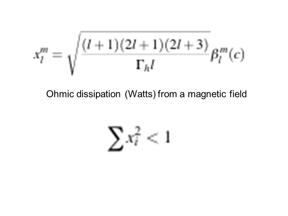
Ohmic dissipation (Watts) from a magnetic field
 from a magnetic field")
40
Independence of x l m ? CLT => much more certain knowledge than expected Dim(X)=∞? Backus=> much more certain knowledge than expected

41
The B field is not infinite dimensional – magnetic dissipation

42
The prior for Ohmic dissipation P(dissipation) Minimum (or no dynamo for last 3.5 Billion years) Maximum (or oceans -> steam) Dissipation
 Minimum (or no dynamo for last 3.5 Billion years) Maximum (or oceans -> steam) Dissipation")
43
P(x 1,x 2,x 3,….x n ) ~ (x 1 2 +x 2 2 +x 3 2 +….x n 2 ) -n/2+1 How to solve this inference problem? Too big for MCMC

Similar presentations


 University.>")


 spatial inference = prediction temporal inference.>")
 Tutorial 7.>")


 Tutorial 6 FLUID KINETMATICS.>")
>")