Download presentation
Presentation is loading. Please wait.

1
http://www.firstcolonialhs.vbschools.com/ap/summer_10_stats.pdf
2
Sta220 - Statistics Mr. Smith Room 310 Class #4

3
Section 2.5-2.6

4
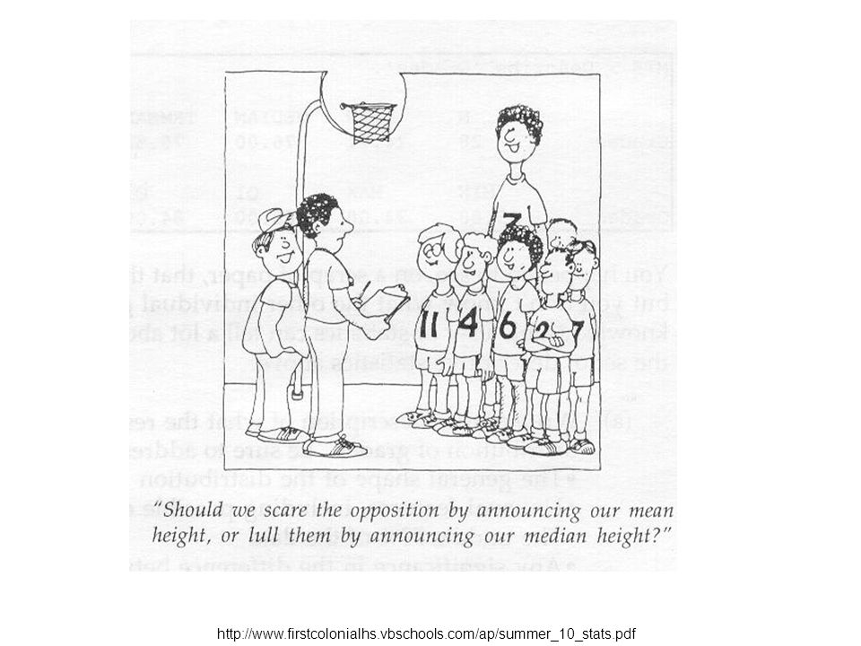
PLAY BALL! Team 1 Heights (Inches) Mean = 75 Median = 76 Mode = 76 Team 2 Heights (Inches) Mean = 75 Median = 76 Mode = 76
 Mean = 75 Median = 76 Mode = 76 Team 2 Heights (Inches) Mean = 75 Median = 76 Mode = 76.")
5
Data sets have the same Mean, Median, and Mode yet clearly differ!

6
Knowledge of the data set’s variability, along with knowledge of its center, can help us visualize the shape of the data set as well as its extreme values.

7
1-7 Lesson Objectives You will be able to: 1.Compute the range of a variable from raw data 2.Compute the variance of a variable from raw data 3.Compute the standard deviation of a variable from raw data 4.Use Chebyshev’s Rule and the Empirical Rule to describe data that are bell shaped

8
Lesson Objective #1-Compute the range of a variable from raw data

9
The simplest measure of variability of a quantitative data set is its range. The range of a quantitative data set is equal to the largest measurement minus the smallest measurement. Range = R = Largest Data Value – Smallest Data Value

10
Team I has range 6 inches, Team II has range 17 inches

11
Copyright © 2013 Pearson Education, Inc.. All rights reserved. Figure 2.19 Response time histograms for two drugs

12
Lesson Objective #2 and #3-Compute the variance and standard deviation of a variable from raw data

14
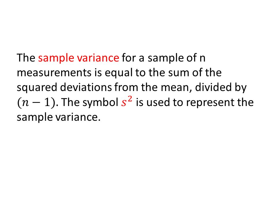
Formula for the Sample variance:

15
Steps to Calculate the Sample Variance:

16
Example of Variance Consider the following sample: 3, 4, 8 Compute the sample variance for this sample.

17
Variance

18
18 Variance

19
Values x MeanDeviationDeviation squared 35-24 451 8539

20
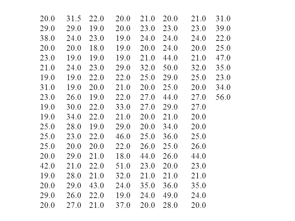
Example The following raw data are the ages of students who completed the student survey during the early fall term 2009.

21
20.0 29.0 38.0 20.0 23.0 21.0 19.0 31.0 23.0 19.0 25.0 20.0 42.0 19.0 20.0 29.0 20.0 31.5 29.0 24.0 20.0 19.0 24.0 19.0 26.0 30.0 34.0 28.0 23.0 20.0 29.0 21.0 28.0 29.0 26.0 27.0 22.0 19.0 23.0 18.0 19.0 23.0 22.0 20.0 19.0 22.0 19.0 22.0 20.0 21.0 22.0 21.0 43.0 22.0 21.0 20.0 19.0 29.0 22.0 21.0 22.0 33.0 21.0 29.0 46.0 22.0 18.0 51.0 32.0 24.0 19.0 37.0 21.0 23.0 24.0 20.0 21.0 32.0 25.0 20.0 27.0 20.0 25.0 26.0 44.0 23.0 21.0 35.0 24.0 20.0 23.0 24.0 44.0 50.0 29.0 25.0 44.0 29.0 21.0 34.0 36.0 25.0 26.0 20.0 21.0 36.0 49.0 28.0 21.0 23.0 24.0 20.0 21.0 32.0 25.0 20.0 27.0 20.0 25.0 26.0 44.0 23.0 21.0 35.0 24.0 20.0 31.0 39.0 22.0 25.0 47.0 35.0 23.0 34.0 56.0
22
StatCrunch

24
Variance Values x MeanDeviationDeviation squared 35-24 451 8539

25
Standard Deviation

26
StatCrunch

27
Symbols for Variance and Standard Deviation The larger the standard deviation, the more variable the data are. The smaller the standard deviation, the less variation there is in the data.

28
To order food at a McDonald’s Restaurant, one must choose from multiple lines, while at Wendy’s Restaurant, one enters a single line. The following data represent the wait time (in minutes) in line for a simple random sample of 30 customers at each restaurant during the lunch hour. For each sample, answer the following: (a) What was the mean wait time? (b) Draw a histogram of each restaurant’s wait time. (c ) Which restaurant’s wait time appears more dispersed? Which line would you prefer to wait in? Why? 3-28
 in line for a simple random sample of 30 customers at each restaurant during the lunch hour. For each sample, answer the following: (a) What was the mean wait time. (b) Draw a histogram of each restaurant’s wait time. (c ) Which restaurant’s wait time appears more dispersed. Which line would you prefer to wait in. Why")
29
http://www.maniacworld.com/Laziness-in-the-Fast-Food-Line.jpg

30
1.500.791.011.660.940.67 2.531.201.460.890.950.90 1.882.941.401.331.200.84 3.991.901.001.540.990.35 0.901.230.921.091.722.00 3.500.000.380.431.823.04 0.000.260.140.602.332.54 1.970.712.224.540.800.50 0.000.280.441.380.921.17 3.082.750.363.102.190.23 Wait Time at Wendy’s Wait Time at McDonald’s

32
(a) The mean wait time in each line is 1.39 minutes.
 The mean wait time in each line is 1.39 minutes.")
33
EXAMPLE Comparing Standard Deviations Determine the standard deviation waiting time for Wendy’s and McDonald’s. Which is larger? Why? Sample standard deviation for Wendy’s: 0.738 minutes Sample standard deviation for McDonald’s: 1.265 minutes 3-33

34
(a) The mean wait time in each line is 1.39 minutes.
 The mean wait time in each line is 1.39 minutes.")
35
Lesson Objective #4-Use Chebyshev’s Rule and the Empirical Rule to describe data that are bell shaped

36
Chebyshev’s Rule applies to any data set, regardless of the shape of the frequency distribution of the data.

37
a. It is possible that very few of the measurements will fall within one standard deviation of the mean. b. At least ¾ of the measurements will fall within two standard deviations of the mean. c. At least 8/9 of the measurements will fall within three standard deviations of the mean.

38
NOTE: Chebyshev’s rule gives the smallest percentages that are mathematically possible. In reality, the true percentages can be much higher than those stated.

39
The empirical rule is a rule of thumb that applies to data sets with frequency distributions that are mound shaped and symmetric as follows: Copyright © 2013 Pearson Education, Inc.. All rights reserved.

40
a.Approximately 68% of the measurements will fall within one standard deviation of the mean. b. Approximately 95% of the measurements will fall within two standard deviation of the mean. c. Approximately 99.7% of the measurements will fall within three standard deviation of the mean. This is know as the 68, 95, and 99.7 Rule.

41
NOTE: Mound-shaped, symmetric distributions is when the mean, median and mode are all about the same.

42
3-42

43
The following histogram is the heights of males who took the statistics 1 student survey for the early fall 2009 to late fall 2010. 3-43 a)Compute the sample mean and standard deviation. Round to one decimal place. b)Draw a histogram to verify the data is bell-shaped. c)Determine the percentage of males that have within 1 standard deviation of the mean, 2 standard deviations from the mean, and 3 standard deviations from the mean according to the Empirical Rule. Student Survey Example
Compute the sample mean and standard deviation. Round to one decimal place. b)Draw a histogram to verify the data is bell-shaped. c)Determine the percentage of males that have within 1 standard deviation of the mean, 2 standard deviations from the mean, and 3 standard deviations from the mean according to the Empirical Rule. Student Survey Example.")
45
70.8 – 3.1 = 67.7 70.8 + 3.1 = 73.9 70.8 – 2(3.1) = 70.8 – 6.2 = 64.6 70.8 + 2(3.1) = 70.8 + 6.2 = 77.0 70.8 – 3(3.1) = 70.8 – 9.3 = 61.5 70.8 + 3(3.1) = 70.8 + 9.3 = 80.1 3-45 68% of the male heights are between 67.7 inches and 73.9 inches 95% of the male heights are between 64.6 inches and 77 inches 99.7% of the male heights are between 61.5 inches and 80.1 inches
 = 70.8 – 6.2 = (3.1) = = – 3(3.1) = 70.8 – 9.3 = (3.1) = = % of the male heights are between 67.7 inches and 73.9 inches 95% of the male heights are between 64.6 inches and 77 inches 99.7% of the male heights are between 61.5 inches and 80.1 inches")
46
70.8 – 3.1 = 67.7 70.8 + 3.1 = 73.9 70.8 – 2(3.1) = 70.8 – 6.2 = 64.6 70.8 + 2(3.1) = 70.8 + 6.2 = 77.0 70.8 – 3(3.1) = 70.8 – 7.8 = 61.5 70.8 + 3(3.1)= 70.8 + 7.8 = 80.1
 = 70.8 – 6.2 = (3.1) = = – 3(3.1) = 70.8 – 7.8 = (3.1)= = 80.1")
47
Rat-in-Maze Experiment Thirty students in an experimental psychology class use various techniques to train a rat to move through a maze. At the end of the course, each student’s rat is timed as it navigates the maze. The results (in minutes) are listed in table below. Determine the faction of the 30 measurements in one-, two- and three-standard deviation, and compare the results with Chebyshev’’s Rule and the Empirical Rule. Copyright © 2013 Pearson Education, Inc.. All rights reserved.
 are listed in table below. Determine the faction of the 30 measurements in one-, two- and three-standard deviation, and compare the results with Chebyshev’’s Rule and the Empirical Rule. Copyright © 2013 Pearson Education, Inc.. All rights reserved..")
48
Data Times (in minutes) of 30 Rats Running through a Maze 1.97.604.023.21.156.064.442.023.373.65 1.742.753.819.708.295.635.214.557.603.16 3.775.361.061.712.474.251.935.152.061.65 Copyright © 2013 Pearson Education, Inc.. All rights reserved.

49
Summary statistics ColumnnMeanVarianceStd. dev.Std. err.MedianMinMax RUNTIME303.74434.83222.19820.40133.510.69.7 :

50
Interval of Interest

52
Compare

Similar presentations


/10=46.7 »Median (50+51)/2=50.5 »mode.>")


