1. CDS 130 - 003 Fall, 2010 Computing for Scientists Scientific Simulation (Sep. 27, 2010 – Oct. 21, 2010) Jie Zhang Copyright ©

2. Motivation Scientific simulation allows one to reproduce the details of a complex scientific system, e.g., physical systems, biological systems It is a new way of scientific research, in additional to traditional experimental and mathematical approaches.

3. Example Merger of the Milky Way: http://video.google.com/videoplay?docid=3671579993993423979# The Milky Way and the Andromeda galaxy will likely fall together and merge within a few billion years. In this speculative simulation, the two galaxies flyby one another, exciting tidal tails and bridges and collide on a second pass finally merging after several convulsions. The last remnants of the smashed spirals show up as shells and ripples surrounding a newborn elliptical galaxy.

4. Example Many scientific simulations are based on so-called Navier-Stokes Equations (Note: do not worry about the math complexity) http://www.cfd-online.com/Wiki/Navier-Stokes_equations Navier-Stokes Equations

5. Example Cellular Blood Flow: http://www.youtube.com/watch?v=o11NDvrZMNs&feature=related The RBCs are modeled as a membrane with hemoglobin inside with a viscosity of 6cP. Each RBC membrane is constructed of linear finite element triangular shells. These shell elements deform due to the fluid-structure interactions with the blood plasma and the hemoglobin.

6. Objectives 1.Mathematical Models 2.Numerical Methods Iteration Differentiation Integration 3.Verification and Validation

7. A Pipeline of Models 1.Domain specialists (e.g., biologists) develop a conceptual representation of the system or a scientific model 2.The domain specialists collaborate with mathematicians to develop a mathematical representation, or mathematical model that corresponds to the science model 3.The domain specialists and mathematicians work with computational scientists to implement the equations and explore the results using a computer, that is to develop a computational model of the mathematical model. 4.The computational methods need to be verified, and the results need to be validated. A common way that science gets done

8. Mathematical Models (Sep. 29, 2010)

9. Example 1 scientific model: Every year your bank account balance increases by 20% Mathematical model: B(next-year) = B(this-year) + 0.2 * B(this-year) Or B(next-year) - B(this-year) = 0.2 * B(this-year)

10. Example 2 scientific model: Every year your bank account balance increases by 20%. Every year you pay a fee of $100 to the bank Mathematical model: B(next-year) = B(this-year) + 0.2 * B(this-year) - 100

11. Example 3 scientific model: Every year your bank account balance doubles Mathematical model: B(next-year) = 2 * B(this-year)

12. Example 4 scientific model: The death rate is 1% and no babies are born Mathematical model: P (next-year) = P(this-year) – 0.01*P(this-year) OR: this year is represented by index I next year is represented by index 2 P(2) = P(1) – 0.01*P(1)

13. Example 5 scientific model: The rabbit birth rate is 10% and no rabbits die Mathematical model: P (next-year) = P(this-year) + 0.1 * P(this-year) Using index “i”, “i” represents this year. In the context of iteration, “I” represents current year P(i+1) = P(i) + 0.1*P(i)

14. Example 5 (cont.) Mathematical model: P(i+1) = P(i) + 0.1*P(i) One instance of simulation: Assuming initial population of 100, find the population in the next five year First year (i=1): P(1) = 100 Second year (i=2): P(2) = P(1) + 0.1*P(1) = 110 Third year (i=3): P(3) = P(2) + 0.1*P(2) = 121 Fourth year (i=4): P(4) = P(3) + 0.1*P(3) = 133 Fifth year (i=5): P(5) = P(4) + 0.1*P(4) = 146

15. Example 5 (cont.) Calculation in Excel >P(1) = 100 >P(2) = P(1) + 0.1*P(1) = 110 >P(3) = P(2) + 0.1*P(2) = 121 >P(4) = P(3) + 0.1*P(3) = 133 >P(5) = P(4) + 0.1*P(4) = 146 >plot(P,’*’) Calculation in Matlab/Octav

16. Example 6 scientific model: The birth rate of rabbits is 10%. The death rate or rabbits is 0.02 times the number of rabbits multiplied by the number of foxes. Mathematical model: R (next-year) = R(this-year) + 0.10*R(this-year) – 0.02*R(this-year)*F(this-year) Use “i” represents the current year R(i+1)=R(i) + 0.10*R(i) – 0.02*R(i)*F(i)

17. Example 7 Scientific model: The death rate of foxes is 10%. The birth rate of foxes is 2% of the number of rabbits multiplied by the number of foxes. Mathematical model: F (next-year) = ?

18. Example 8 scientific model: The birth rate of rabbits is 10%. The death rate or rabbits is 0.02 times the number of rabbits multiplied by the number of foxes. The death rate of foxes is 10%. The birth rate of foxes is 2% of the number of rabbits multiplied by the number of foxes. Mathematical model: R(i+1)=R(i) + 0.10*R(i) – 0.02*R(i)*F(i) F(i+1)=F(i) - 0.10*R(i) + 0.02*R(i)*F(i)

19. Example 8 (cont.) Mathematical model: R(i+1)=R(i) + 0.10*R(i) – 0.02*R(i)*F(i) F(i+1)=F(i) - 0.10*F(i) + 0.02*R(i)*F(i) One instance of simulation: Initial population of rabbits is 100, and that of foxes is 20. What are the population in the second year? >R(1) = 100 >F(1) = 50 >R(2)=R(1) + 0.10*R(1) – 0.02*R(1)*F(1) = 70 >F(2)=F(1) - 0.10*F(1) + 0.02*F(1)*R(1) = 58

20. Simulation Project A closed system (e.g., Rabbits and Foxes on an island) Change in number of rabbits per year increases in proportion to the number of rabbits (breeding like rabbits!) – the birth rate of prey decreases in proportion to (the number of rabbits) x (number of foxes) - the death rate of prey due to interaction Does not depend on rabbits dying of natural death Change in number of foxes per year decreases in proportion to the number of foxes (more competition for food) – the death rate of predator increases in proportion to (the number of rabbits) x (the number of foxes) – the birth rate of predator due to interaction Predator – Prey Model http://home.messiah.edu/~deroos/CSC171/PredPrey/PRED.htm

21. Simulation Project Predator – Prey Model Simulation: Given (1) initial rabbit population, (2) initial fox population, (3) rabbit birth rate, (4) rabbit death rate due to interaction, (5) fox death rate, (5) fox birth rate due to interaction. You need to find out how the population change with time?

22. Numerical Method - Iteration (Oct. 5, 2010)

23. Iteration Iteration is the most fundamental numerical method to solve the mathematical model that represents a dynamic scientific system, the evolution or the time change of the system. Used for solving differential equations e.g., knowing the rate of change of the population Used for solving integration equations e.g., total area enclosed by a Gaussian function X(i+1) = X(i) + f(X(i))

24. Iteration The output of current iteration is used as the input of the next iteration i: the sequence number of the iteration, representing the independent variable “time”, e.g., year in population growth N: total number of iterations X: the dependence variable, an unknown function, but the model seeks to find f(X(i)): the known function representing the rate of change >for i=1:N >X(i+1) = X(i) + f(X(i)); >end

25. Example 1 scientific model: The human population grows at an annual rate of 2% Mathematical model: P (i+1) = P(i) + 0.02 * P(i) Question: In year 2000, the population is 6.0 billion. What are the populations in the next five years? Work this out with the tools available to you: manual, calculator, excel, and program.

26. Example 1 >P(1) = 6.0 >for i=1:5 >P(i+1)=P(i)+0.02*P(i); >end >P >plot(P,’*’) Year 2000: 6.00 Year 2001: 6.12 Year 2002: 6.24 Year 2003: 6.37 Year 2004: 6.49 Year 2005: 6.62

27. Example 1 Question: In year 2000, the population is 6.0 billion. What about the population in the next 200 years? What is the population in year 2200? Work this out with the tools available to you: manual, calculator, excel, and program.

28. Example 1 >P(1) = 6.0 >for i=1:199 >P(i+1)=P(i)+0.02*P(i); >end >P(199) >plot(P,’*’) >xlabel(‘Year from 2000’) >ylabel(‘Population (billion)’) >title(‘Population Growth’) >cd(‘~’) >print –dpng ‘population.png’ The answer is: the population is 302.60 billion in year 2200.

29. Example 1

30. Example 2 Mathematical model of Predator-Prey scientific model R(i+1)=R(i) + 0.10*R(i) – 0.002*R(i)*F(i) F(i+1)=F(i) - 0.10*F(i) + 0.002*R(i)*F(i) Question: Initial population of rabbits is 100, and that of foxes is 10. What are their populations in the next 10 years? >R(1) = 100 >F(1) = 10 >R(2)=R(1) + 0.10*R(1) – 0.002*R(1)*F(1) = 108 >F(2)=F(1) - 0.10*F(1) + 0.002*F(1)*R(1) = 11 >R(3)=… >F(3)=… >……..

31. Example 2 >R(1) = 100 >F(1)=10 >for i=1:10 >R(i+1)=R(i)+0.10*R(i)-0.002*R(i)*F(i); >F(i+1)=F(i)-0.10*F(i)+0.002*R(i)*F(i); >end >R >F >plot((R) >hold >plot(F) >print –dpng ‘predator_prey.png’

32. Example 2

33. Differential Equations (Oct. 7, 2010)

34. Differential Equations Differential equations play an important role in modelling virtually every physical, technical, or biological process, from celestial motion, to bridge design, to interactions between neurons (http://en.wikipedia.org/wiki/Differential_equation)

35. Differential Equations A differential equation is a mathematical equation for an unknown function of one or several variables that relates its derivatives and the function It is used to describe a dynamic system, in which the time rate of change is well defined

36. Example 1 scientific model: The human population grows at an annual rate of 2% -The rate of change is known -The population evolution is unknown, but described by the following differential equation dP/dt: the rate of change of the population P: the unknown function P, a dependent variable of t t: time, the independent variable dP: differential of P, or change of P dt: differential of t, or change of t

37. Example 1 Δt = 10 years, only know population change every 10 years Δt = 1 year, only know population change every 1 years Δt = 1 day, can calculate population change on daily basis The smaller the time interval, the more accurate the result.

38. Example 1 Differentiation to Iteration

39. Example 1 Iteration to Differentiation

40. Example 2 Newton’s Law of Cooling: A scientific law is often expressed in differential equations, for good reasons The cooling rate of an object is proportional to the temperature difference between the object and the ambient temperature

41. Example 2 Question: An iron bar is heated to 1000°C. Assume the cooling rate is 0.2 min -1, and the ambient temperature is 30°C. At approximately what time (in unit of minute) does the temperature equal one-half of the initial temperature after the iron bar is allowed to cool?

42. Example 2 Convert differential equation to iteration

43. Example 2 >cd(‘~’) >edit cooling.m >cooling >print –dpng ‘cooling.png’

44. function [T] = cooling () T(1)=1000 % initial temperature Ta=30 % ambient temperature q = 0.2 % cooling coefficient %guess the iteration needed %N = 1000 % iteration 1000 times, or calculate up to 1000 minutes N=50 %second guess of appropriate iteration number %start the iteration calculation using for loops for i=1:N T(i+1)=T(i)-q*(T(i)-Ta); endfor plot(T,'*') xlabel('Time (min)') ylabel('Temperature (deg)') title('cooling curve') endfunction “cooling.m”

45. Example 2 Answer: It takes about 4.5 minutes to cool down to the half temperature

46. Example 3 Mathematical model of Predator-Prey scientific model R(i+1)=R(i) + 0.10*R(i) – 0.002*R(i)*F(i) F(i+1)=F(i) - 0.10*F(i) + 0.002*R(i)*F(i) Mathematical notation in differential equations:

47. Example 3 Question: Initial population of rabbits is 100, and that of foxes is 10. What are their populations in the next 50 years? 1.Use a program file to save all the code 2.Use variables to represent the coefficients 3.run the program file

48. Differential Equations (continued): Interval and Sub-interval (Oct. 14, 2010)

49. Interval and Sub-interval In numerical simulation, one has to specify the calculation interval and sub-interval Interval is the domain of the calculation In the population example, if you are asked to calculate the population in the next 10 years, what is the interval or domain of the calculation Answer: from year 1 to year 10, or i=[1:10] in the iteration format Answer: time t in [1,10], or from 1 to 10 in the differentiation format Population Example:

50. Sub-interval Sub-interval is the step-size in each iteration of the numerical calculation In the population example, so far we have always assumed that the sub-interval is 1 year That is, from i to i+1, the time interval is one year However, one can choose a different sub-interval, for instance, one month This can be used to study the population change on a monthly base In the differential notation, dt is formerly defined as infinitely small time interval Population Example:

51. Differentiation Equation to Iteration Equation Sub-interval In the conversion, we’ve made the following approximations (1) Differentiation dt is replaced by finite difference Δt (the time step, or the sub-interval); Correspondingly, dP replaced by ΔP (2) Assuming the sub-interval to be 1; in this example, means one year

52. Question to think? What if you want to study the population change on a finer time resolution, say from month to month? Sub-interval You have to change the step size: Δt = 1/12 year, or one month One iteration from i to i+1 is now one month, instead of one year The rate of change of the population is now (0.02/12) for one month

53. Example >P(1)=6.0 >for i=[1:2] >P(i+1)=P(i)+0.2*P(i); >end Δt = 1 (year) two iteration Δt = 1/12 (year) 24 iteration Question: Given initial population of 6.0 billion, what is the population in the beginning of the third year? P = 6.2424 >P(1)=6.0 >for i=[1:24] >P(i+1)=P(i)+(0.2/12)*P(i); >end P = 6.2447 The two results are close, but different!

54. The Effects of Sub-interval Smaller sub-interval requires more steps of calculation But, smaller sub-interval provides more detailed evolution Further, smaller sub-interval provides more accurate results, e.g., fully illustrated in the context of integration

55. Integration (Oct. 14, 2010) (Oct. 19, 2010)

56. Integration Integration is like the opposite operation of the differentiation Differentiation: the rate of change of a function, e.g. given what is f(i+1)-f(i) Integration: the total sum of a function over a domain e.g., find what is f(i+1)+f(i)

57. Primitive Integration Primitive integration method has long been used by ancient mathematicians A good example is to find the area size of a circle, that leads to the discovery of π The piece-wise approach Count the small tiles with known size The smaller the tile, the more accurate the circular area, thus the π In other words, the smaller the sub- interval, the more the accuracy S = π r 2

58. Mathematical notation f(x): the integrant, the function of concern F: the total value of integration [a, b]: the interval of integration a: lower limit, b: upper limit dx: the sub-interval of integration. Infinitely small in calculus

59. Integration: geometric meaning Integration can be defined as the total area enclosed by the function between the integration interval

60. Integration: Piece-wise Approach The total area is approximated by the sum of the sizes of the rectangles (L1+L2+L3….). The size of each rectangle can be easily calculated over the sub-interval: L i = f(x i ) * Δx

61. Integration to Iteration

62. Example: f(x)=x Question: integrate the function f(x)=x from the interval x=0 to x=5. It is equivalent to find the area of the triangle with the base of 5 and the height of 5. The area is expected to be 12.5

63. Example: f(x)=x Using 5 rectangles: N=5, The approximate value is smaller than the true value

64. Example: f(x)=x Using 10 rectangles: N=10, sub-interval Δx=0.5 N=10; %number of rectangles, or iteration a=0; % lower limit b=5.0; % upper limit del_x=(b-a)/N; %the sub-interval x1=a; F(1)=x1*del_x; for i=[2:N] xi=x1+(i-1)*del_x; F(i)=F(i-1)+xi*del_x; end “area1.m” F=11.25

65. Example: f(x)=x Using 20 rectangles: N=20, sub-interval Δx=0.25 F=11.875 Using 50 rectangles: N=50, sub-interval Δx=0.10 F=12.25 Using 500 rectangles: N=500, sub-interval Δx=0.01 F=12.475 Using 5000 rectangles: N=5000, sub-interval Δx=0.001 F=12.4975 Therefor, the smaller the sub-interval, the better the accuracy

66. Example: f(x)=x 2 Question: integrate the function f(x)=x 2 from the interval x=0 to x=5. Find the value when the number of sub-intervals is chosen to be (1)N=5 (2)N=10 (3)N=100 (4)N=1000

67. Example: f(x)=x 2 Using 5 rectangles: N=5, This approximate value is smaller than the true value

68. Integration Question: How does the integration accuracy depend on the size of the sub-interval? Why?

69. Verification and Validation (Oct. 19, 2010)

70. Scientific Method Four essential elements of a scientific method: 1.Characterization: observation and measurement 2.Hypothesis 3.Prediction 4.Testing It is an iterative process until the prediction is consistent with the observation The hypothesis becomes a theory. Verification and validation is an integral part of the scientific method.

71. Verification Versus Validation For the scientific method that involves scientific simulation, the testing has two basic stages: 1.Verification: Are you solving the equations right? 2.Validation: Are you solving the right equation? Verification is to make sure that your computer program is correct Validation is to make sure that your scientific hypothesis, or the scientific model, is correct. A scientific model is often specified by 1.Equations 2.Adjustable parameters, e.g., growth rate

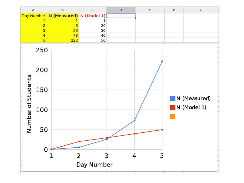
72. Example We use a study on flu outbreak to demonstrate the scientific method and the validation process. Data are based on the article http://dx.doi.org/10.1136/bmj.1.6112.586 In a school of 762 students, the first flu case was reported on Jan. 22. There were 6 cases found on Jan. 23. The number of infected students grew to 26, 73 and 222 in the following three days. Construct a scientific model to explain the outbreak?

73. Characterization (Step 1) Observe the phenomena Collect the data Analyze the data

74. Hypothesis (Step 2) Forming the hypothesis Model 1 The number of students infected equals 10 times the day number since the outbreak, with day number = 1 corresponding to the day the first student was infected.

75. Prediction (Step 3) Formulation of a predictive test Create a mathematic model Implement and run the computational model Obtain the predictive result

77. Testing (Step 4) Verify that the calculation is done right Do sanity checks: Does the simulation predict behavior that would never happen in reality? Does population ever go negative? Does the mass stay positive? Compare the model prediction with existing data Determine if the prediction “matches” the observation Apparently, the match is “not good” How to determine “not good” or “good”. This will be explored in the next chapter.

78. Model 2: Repeat step 2, 3 and 4 with different scientific model

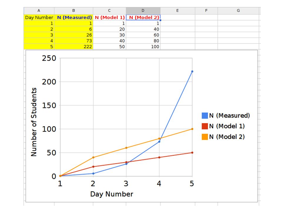
79. Hypothesis (Step 2) Forming the hypothesis Model 2 The number of students infected equals 20 times the day number since the outbreak, with day number = 1 corresponding to the day the first student was infected.

80. Prediction (Step 3) Formulation of a predictive test Create a mathematic model Implement and run the computational model Obtain the predictive result

82. Testing (Step 4) Again, the model prediction does not fit the observed data Need a better model Need to further study the data Need to think about the scientific justification of the model

83. Model 3: Repeat step 2, 3 and 4 with different scientific model

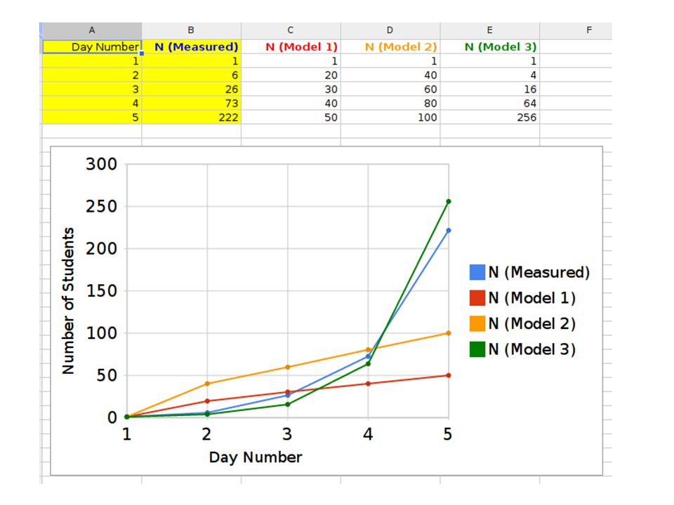
84. Hypothesis (Step 2) Forming the hypothesis Model 3 The number of new people infected on a given day is proportional to the number of people infected on the previous day. The proportion rate is an adjustable parameter. In this model, it is assumed to be 3.

85. Prediction (Step 3) Formulation of a predictive test Create a mathematic model Implement and run the computational model Obtain the predictive result

87. Testing (Step 4) This model is “good” It is a good representation of the observation Caveats It is not an exact representation, but a good approximation of the observations It is only validated on the initial stage of an outbreak. It is not a model to explain the long term evolution.

88. Scientific Method It is an iterative process. One needs to re- form the hypothesis and re-test the result. 1. Characterizat ion 2. Hypothesis 3. Prediction 4. Testing

89. The end (Oct. 21, 2010)