Download presentation
Presentation is loading. Please wait.

1
A Bit of Progress in Language Modeling Extended Version
Presented by Louis-Tsai Speech Lab, CSIE, NTNU

2
Introduction Overview
LM is the art of determining the probability of a sequence of words Speech recognition, optical character recognition, handwriting recognition, machine translation, spelling correction Improvements Higher-order n-grams Skipping models Clustering Caching Sentence-mixture models

3
Introduction Technique introductions
The goal of a LM is to determine the probability of a word sequence w1…wn, P(w1…wn) Trigram assumption
 Trigram assumption.")
4
Introduction Technique introductions
C(wi-2wi-1wi) represent the number of occurrences of wi-2wi-1wi in the training corpus, and similarly for C(wi-2wi-1) There are many three word sequences that never occur, consider the sequence “party on Tuesday”, what is P(Tuesday | party on)?
 represent the number of occurrences of wi-2wi-1wi in the training corpus, and similarly for C(wi-2wi-1) There are many three word sequences that never occur, consider the sequence party on Tuesday , what is P(Tuesday | party on)")
5
Introduction Smoothing
The training corpus might not contain any instances of the phrase, so C(party on Tuesday) would be 0, while there might still be 20 instances of the phrase “party on” P(Tuesday | party on) = 0 Smoothing techniques take some probability away from some occurrences Imagine we have “party on Stan Chen’s birthday” in the training data and occurs only one time
 would be 0, while there might still be 20 instances of the phrase party on P(Tuesday | party on) = 0. Smoothing techniques take some probability away from some occurrences. Imagine we have party on Stan Chen’s birthday in the training data and occurs only one time.")
6
Introduction Smoothing
By taking some probability away from some words, such as “Stan” and redistributing it to other words, such as “Tuesday”, zero probabilities can be avoided Katz smoothing Jelinek-Mercer smoothing (deleted interpolation) Kneser-Ney smoothing
 Kneser-Ney smoothing.")
7
Introduction Higher-order n-grams
The most obvious extension to trigram models is to simply move to higher-order n-grams, such as four-grams and five-grams There is a significant interaction between smoothing and n-gram order : higher-order n-grams work better with Kneser-Ney smoothing than with some other methods, especially Katz smoothing

8
Introduction Skipping
We condition on a different context than the previous two words Instead computing P(wi|wi-2wi-1) of computing P(wi|wi-3wi-2)
 of computing P(wi|wi-3wi-2)")
9
Introduction Clustering
Clustering (classing) models attempt to make use of the similarities between words If we have seen occurrences of phrases like “party on Monday” and “party on Wednesday” then we might imagine that the word “Tuesday” is also likely to follow the phrase “party on”
 models attempt to make use of the similarities between words. If we have seen occurrences of phrases like party on Monday and party on Wednesday then we might imagine that the word Tuesday is also likely to follow the phrase party on")
10
Introduction Caching Caching models make use of the observation that if you use a word, you are likely to use it again

11
Introduction Sentence Mixture
Sentence Mixture models make use of the observation that there are many different sentence types, and that making models for each type of sentence may be better than using one global model

12
Introduction Evaluation
A LM that assigned equal probability to 100 words would have perplexity 100

13
Introduction Evaluation
In general, the perplexity of a LM is equal to the geometric average of the inverse probability of the words measured on test data:

15
Introduction Evaluation
“true” model for any data source will have the lowest possible perplexity The lower the perplexity of our model, the closer it is, in some sense, to the true model Entropy, which is simply log2 of perplexity Entropy is the average number of bits per word that would be necessary to encode the test data using an optimal coder

16
Introduction Evaluation
reduction entropy .01 .1 .16 .2 .3 .4 .5 .75 1 perplexity 0.69% 6.7% 10% 13% 19% 24% 29% 41% 50% entropy : 54 perplexity : 32 % entropy : 54.5 perplexity : 32 %

17
Introduction Evaluation
Experiments corpus: 1996 NAB Experiments performed at 4 different training data sizes :100K words, 1M words, 10M words, 284M words Heldout and test data taken from the 1994 WSJ Heldout data: 20K words Test data: 20K words Vocabulary: 58,546 words

18
Smoothing simply interpolation
where 0≦,≦1 In practice, the uniform distribution are also interpolated this ensures that no word is assigned probability 0

19
Smoothing Katz smoothing
Katz smoothing is based on the Good-Turing formula Let nr represent the number of n-grams that occur r times discount :

20
Smoothing Katz smoothing
(r+1)nr+1=0 Let N represent the total size of the training set, this left-over probability will be equal to n1/N Sum=n1
nr+1=0. Let N represent the total size of the training set, this left-over probability will be equal to n1/N. Sum=n1.")
21
Smoothing Katz smoothing
Consider a bigram model of a phrase such as Pkatz(Francisco | on). Since the phrase San Francisco is fairly common, the unigram probability will also be fairly high. This means that using Katz smoothing, the probability will also be fairly high. But, the word Francisco occurs in exceedingly few contexts, and its probability of occurring in a new one is very low
. Since the phrase San Francisco is fairly common, the unigram probability will also be fairly high. This means that using Katz smoothing, the probability will also be fairly high. But, the word Francisco occurs in exceedingly few contexts, and its probability of occurring in a new one is very low.")
22
Smoothing Kneser-Ney smoothing
KN smoothing uses a modified backoff distribution based on the number of contexts each word occurs in, rather than the number of occurrences of the word. Thus, the probability PKN(Francisco | on) would be fairly low, while for a word like Tuesday that occurs in many contexts, PKN(Tuesday | on) would be relatively high, even if the phrase on Tuesday did not occur in the training data
 would be fairly low, while for a word like Tuesday that occurs in many contexts, PKN(Tuesday | on) would be relatively high, even if the phrase on Tuesday did not occur in the training data.")
23
Smoothing Kneser-Ney smoothing
Backoff Kneser-Ney smoothing where |{v|C(vwi)>0}| is the number of words v that wi can occur in the context, D is the discount, is a normalization constant such that the probabilities sum to 1
>0}| is the number of words v that wi can occur in the context, D is the discount, is a normalization constant such that the probabilities sum to 1.")
24
Smoothing Kneser-Ney smoothing
V={a,b,c,d} b b a a c c d a a b b b b c c a a b c c b c c d a d d c

25
Smoothing Kneser-Ney smoothing
Interpolated models always combine both the higher-order and the lower-order distribution Interpolated Kneser-Ney smoothing where (wi-1) is a normalization constant such that the probabilities sum to 1
 is a normalization constant such that the probabilities sum to 1.")
26
Smoothing Kneser-Ney smoothing
Multiple discounts, one for one counts, another for tow counts, and another for three or more counts. But it have too many parameters Modified Kneser-Ney smoothing

27
Smoothing Jelinek-mercer smoothing
Combines different N-gram orders by linearly interpolating all three models whenever computing trigram

28
Smoothing absolute discounting
Absolute discounting subtracting a fixed discount D<=1 from each nonzero count

29
Witten-Bell Discounting
Key Concept—Things Seen Once: Use the count of things you’ve seen once to help estimate the count of things you’ve never seen So we estimate the total probability mass of all the zero N-grams with the number of types divided by the number of tokens plus observed types: N : the number of tokens T : observed types

30
Witten-Bell Discounting
T/(N+T) gives the total “probability of unseen N-grams”, we need to divide this up among all the zero N-grams We could just choose to divide it equally Z is the total number of N-grams with count zero
 gives the total probability of unseen N-grams , we need to divide this up among all the zero N-grams. We could just choose to divide it equally. Z is the total number of N-grams with count zero.")
31
Witten-Bell Discounting
Alternatively, we can represent the smoothed counts directly as:

32
Witten-Bell Discounting

33
Witten-Bell Discounting
For bigram T: the number of bigram types, N: the number of bigram token

34
20 words per sentence

35
Higher-order n-grams Trigram P(wi|wi-2wi-1) five-gram P(wi|wi-4wi-3wi-2wi-1) In many cases, no sequence of the form wi-4wi-3wi-2wi-1 will have been seen in the training data backoff to or interpolation with four-grams, trigrams, bigrams, or even unigrams But in those cases where such a long sequence has been seen, it may be a good predictor of wi

36
0.06 0.02 0.01 284,000,000

37
Higher-order n-grams As we can see, the behavior for Katz smoothing is very different than the behavior for KN smoothing the main cause of this difference was backoff smoothing techniques, such as Katz smoothing, or even the backoff version of KN smoothing Backoff smoothing techniques work poorly on low counts, especially one counts, and that as the n-grams order increases, the number of one counts increases

38
Higher-order n-grams Katz smoothing has its best performance around the trigram level, and actually gets worse as this level is exceeded KN smoothing is essentially monotonic even through 20-grams The plateau point for KN smoothing depends on the amount of training data available small (100,000 words) at trigram level full (284 million words) at 5 to 7 gram (6-gram has .02 bits better than 5-gram, 7-gram has .01 bits better than 6-gram)
 at trigram level full (284 million words) at 5 to 7 gram. (6-gram has .02 bits better than 5-gram, 7-gram has .01 bits better than 6-gram)")
39
Skipping When considering a 5-gram context, there are many subsets of the 5-gram we could consider, such as P(wi|wi-4wi-3wi-1) or P(wi|wi-4wi-2wi-1) If have never seen “Show John a good time” but we have seen “Show Stan a good time”. A normal 5-gram predicting P(time | show John a good) would back off to P(time | John a good) and from there to P(time | a good), which would have a relatively low probability A skipping model of the from P(wi|wi-4wi-2wi-1) would assign high probability to P(time | show ____ a good)
 would back off to P(time | John a good) and from there to P(time | a good), which would have a relatively low probability. A skipping model of the from P(wi|wi-4wi-2wi-1) would assign high probability to P(time | show ____ a good)")
40
Skipping P(wi|wi-2wi-1) + P(wi|wi-3wi-1) +(1--) P(wi|wi-3wi-2)
These skipping 5-grams are then interpolated with a normal 5-gram, forming models such as where 0≦ ≦1 and 0 ≦ ≦1 and 0 ≦ (1--) ≦1 Another (and more traditional) use for skipping is as a sort of poor man’s higher order n-gram. One can, for instance, create a model of the form no component probability depends on more than two previous words but the overall probability is 4-gram-like, since it depends on wi-3, wi-2, and wi-1 P(wi|wi-4wi-3wi-2wi-1) + P(wi|wi-4wi-3wi-1) +(1--) P(wi|wi-4wi-2wi-1) P(wi|wi-2wi-1) + P(wi|wi-3wi-1) +(1--) P(wi|wi-3wi-2)
 ≦1. Another (and more traditional) use for skipping is as a sort of poor man’s higher order n-gram. One can, for instance, create a model of the form no component probability depends on more than two previous words but the overall probability is 4-gram-like, since it depends on wi-3, wi-2, and wi-1. P(wi|wi-4wi-3wi-2wi-1) + P(wi|wi-4wi-3wi-1) +(1--) P(wi|wi-4wi-2wi-1) P(wi|wi-2wi-1) + P(wi|wi-3wi-1) +(1--) P(wi|wi-3wi-2)")
41
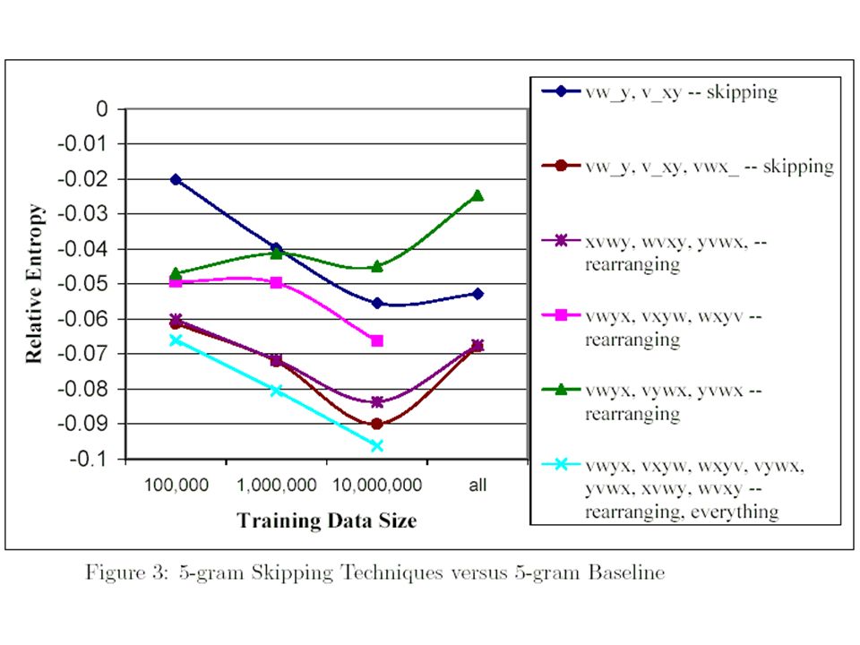
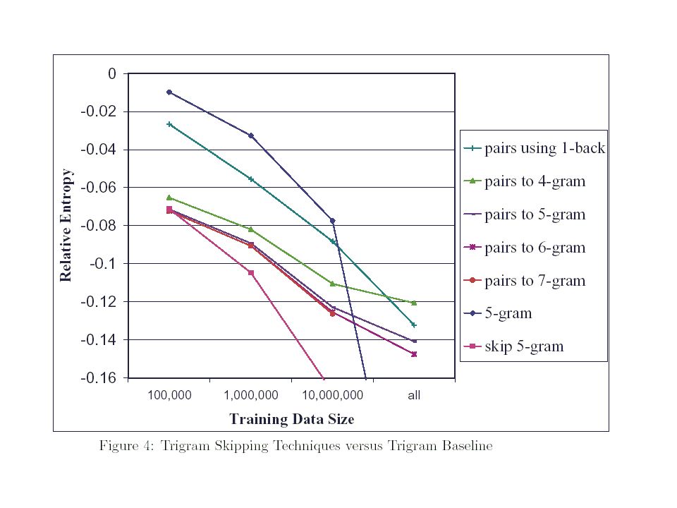
Skipping For a 5-gram skipping experiments, all contexts depended on at most the previous four words, wi-4, wi-3, wi-2,and wi-1, but used the four words in a variety of ways For readability and conciseness, we define v = wi-4, w = wi-3, x = wi-2, y = wi-1

43
Skipping First model interpolated dependencies on vw_y and v_xy does not work well on the smallest training data size, but is competitive for larger ones In second model, we add vwx_ into first model roughly .02 to .04 bits over the first model Next, adding back in the dependencies on the missing words, xvwy, wvxy, and yvwx; that is, all models depended on the same variables, but with the interpolation order modified e.g., by xvwy, we refer to a model of the form P(z|vwxy) interpolated with P(z|vw_y) interpolated with P(z|w_y) interpolated with P(z|y) interpolated with P(z)
 interpolated with P(z|vw_y) interpolated with P(z|w_y) interpolated with P(z|y) interpolated with P(z)")
44
Skipping Interpolating together vwyx, vxyw, wxyv (base on vwxy) This model puts each of the four preceding words in the last position for one component this model does not work as well as the previous two, leading us to conclude that the y word is by far the most important
 This model puts each of the four preceding words in the last position for one component this model does not work as well as the previous two, leading us to conclude that the y word is by far the most important.")
45
Skipping Interpolating together vwyx, vywx, yvwx, which put the y word in each possible position in the backoff model this was overall the worst model, reconfirming the intuition that the y word is critical Finally we interpolating together vwyx, vxyw, wxyv, vywx, yvwx, xvwy, wvxy the result is a marginal gain – less than 0.01 bits – over the best previous model

47
Skipping 1-back word (y) xy, wy, vy, uy and ty
4-gram level : xy, wy and wx The improvement over 4-gram pairs was still marginal

48
Clustering Consider a probability such as P(Tuesday | party on)
Perhaps the training data contains no instances of the phrase “party on Tuesday”, although other phrase such as “party on Wednesday” and “party on Friday” do appear We can put words into classes, such as the word “Tuesday” into the class WEEKDAY P(Tuesday | party on WEEKDAY)
")
49
Clustering When each word belongs to only one class, which is called hard clustering, this decomposition is a strict equality a fact that can be trivially proven Let Wi represent the cluster of word wi (1)
")
50
Clustering Since each word belongs to a single cluster, P(Wi|wi) = 1
(2) (2) 代入 (1) 中: (3) predictive clustering
 (2) 代入 (1) 中: (3) predictive clustering.")
51
Clustering Another type of clustering we can do is to cluster the words in the contexts. For instance, if “party” is in the class EVENT and “on” is in the class PREPOSITION, then we could write or more generally Combining (4) with (3) we get (4) (5) fullibm clustering
 with (3) we get. (4) (5) fullibm clustering.")
52
Clustering Use the approximation P(w|Wi-2Wi-1W) = P(w|W) to get fullibm clustering uses more information than ibm clustering, we assumed that it would lead to improvements (goodibm) (6) ibm clustering
 = P(w|W) to get fullibm clustering uses more information than ibm clustering, we assumed that it would lead to improvements (goodibm) (6) ibm clustering.")
53
Clustering index clustering
(7) index clustering Backoff/interpolation go from P(Tuesday| party EVENT on PREPOSITION) to P(Tuesday| EVENT on PREPOSITION) to P(Tuesday| on PREPOSITION) to P(Tuesday| PREPOSITION) to P(Tuesday) since each word belongs to a single cluster redundant
 index clustering. Backoff/interpolation go from P(Tuesday| party EVENT on PREPOSITION) to P(Tuesday| EVENT on PREPOSITION) to P(Tuesday| on PREPOSITION) to P(Tuesday| PREPOSITION) to P(Tuesday) since each word belongs to a single cluster redundant.")
54
Clustering C(party EVENT on PREPOSITION) = C(party on) C(EVENT on PREPOSITION) = C(EVENT on) We generally write an index clustered model as fullibmpredict clustering

55
Clustering indexpredict, combining index and predictive
combinepredict, interpolating a normal trigram with a predictive clustered trigram

56
Clustering allcombinenotop, which is an interpolation of a normal trigram, a fullibm-like model, an index model, a predictive model, a true fullibm model, and an indexpredict model normal trigram fullibm-like index midel predictive true fullibm indexpredict

57
Clustering allcombine, interpolates the predict-type models first at the cluster level, before interpolating with the word level model normal trigram fullibm-like index midel predictive true fullibm indexpredict

58
baseline

59
Clustering The value of clustering decreases with training data increases, since clustering is a technique for dealing with data sparseness ibm clustering consistently works very well

61
Clustering In Fig.6 we show a comparison of several techniques using Katz smoothing and the same techniques with KN smoothing. The results are similar, with same interesting exceptions : Indexpredict works well for the KN smoothing model, but very poorly for the Katz smoothed model. This shows that smoothing can have a significant effect on other techniques, such as clustering

62
Other ways to perform Clustering
Cluster groups of words instead of individual words could compute For instance, in a trigram model, one could cluster contexts like “New York” and “Los Angeles” as “CITY”, and “on Wednesday” and “late tomorrow” as “TIME”

63
Finding Clusters There is no need for the clusters used for different positions to be the same ibm clustering P(wi|Wi)*P(Wi|Wi-2Wi-1) Wi cluster = predictive cluster, Wi-1 and Wi-2 = conditional cluster The predictive and conditional clusters can be different, consider words a and an, in general, a and an can follow the same words, and so, for predictive clustering, belong in the same cluster. But, there are very few words that can follow both a and an – so for conditional clustering, they belong in different clusters
*P(Wi|Wi-2Wi-1) Wi cluster = predictive cluster, Wi-1 and Wi-2 = conditional cluster. The predictive and conditional clusters can be different, consider words a and an, in general, a and an can follow the same words, and so, for predictive clustering, belong in the same cluster. But, there are very few words that can follow both a and an – so for conditional clustering, they belong in different clusters.")
64
Finding Clusters The clusters are found automatically using a tool that attempts to minimize perplexity For the conditional clusters, we try to minimize the perplexity of training data for a bigram of the form P(wi|Wi-1), which is equivalent to maximizing
, which is equivalent to maximizing.")
65
Finding Clusters For the predictive clusters, we try to minimize the perplexity of training data of P(Wi|wi-1)*P(wi|Wi) P(Wiwi)=P(Wi|wi)P(wi) P(Wi|wi) = 1 P(wi-1Wi)=P(wi-1|Wi)P(Wi)
=P(Wi|wi)P(wi) P(Wi|wi) = 1. P(wi-1Wi)=P(wi-1|Wi)P(Wi)")
66
Caching If a speaker uses a word, it is likely that he will use the same word again in the near future We could form a smoothed bigram or trigram from the previous words, and interpolate this with the standard trigram where Ptricache(w|w1…wi-1) is a simple interpolated trigram model, using counts from the preceding words in the same document
 is a simple interpolated trigram model, using counts from the preceding words in the same document.")
67
Caching When interpolating three probabilities P1(w), P2(w), and P3(w), rather than use we actually use This allows us to simplify the constraints of the search
, P2(w), and P3(w), rather than use we actually use This allows us to simplify the constraints of the search.")
68
Caching Conditional caching : weight the trigram cache differently depending on whether or not we have previously seen the context

69
Caching Assume that the more data we have, the more useful each cache is. Thus we make , and be linear functions of the amount of data in the cache Always set maxwordsweight to at or near 1,000,000 while assigning multiplier to a small value (100 or less)
")
70
Caching Finally, we can try conditionally combining unigram, bigram, and trigram caches

72
Caching As can be seen, caching is potentially one of the most powerful techniques we can apply, leading to performance improvements of up to 0.6 bits on small data. Even on large data, the improvement is still substantial, up to 0.23 bits On all data size, the n-gram caches perform substantially better than the unigram cache, but which version of the n-gram is used appears to make only a small difference

73
Caching It should be noted that all of these results assume that the previous words are known exactly In a speech recognition system, it is possible for a cache to “look-in” error if “recognition speech” “wreck a nice beach”, later, “speech recognition” “beach wreck ignition” since the probability of “beach” will be significantly raised

74
Sentence Mixture Models
There may be several different sentence types within a corpus; these types could be grouped by topic, or style, or some other criterion In WSJ data, we might assume that there are three types: financial market sentences (with a great deal of numbers and stock name), business sentences (promotions, demotions, mergers) and general news stories Of course, in general, we do not know the sentence type until we have heard the sentence. Therefore, instead, we treat the sentence type as a hidden variable
, business sentences (promotions, demotions, mergers) and general news stories. Of course, in general, we do not know the sentence type until we have heard the sentence. Therefore, instead, we treat the sentence type as a hidden variable.")
75
Sentence Mixture Models
Let sj denote the condition that the sentence under consideration is a sentence of type j. Then the probability of the sentence, given that it is of type j can be written as Let s0 be a special context that is always true Let there be S different sentence types (4≦S≦8); let 0…S be sentence interpolation parameters, that
; let 0…S be sentence interpolation parameters, that.")
76
Sentence Mixture Models
The overall probability of a sentence w1…wn is Eq (8) can be read as saying that there is a hidden variable, the sentence type; the prior probability for each sentence type is j The probability P(wi|wi-2wi-1sj) may suffer from data sparsity, so they are linearly interpolated with the global model P(wi|wi-2wi-1) (8)
 can be read as saying that there is a hidden variable, the sentence type; the prior probability for each sentence type is j. The probability P(wi|wi-2wi-1sj) may suffer from data sparsity, so they are linearly interpolated with the global model P(wi|wi-2wi-1) (8)")
77
Sentence Mixture Models
Sentence types for the training data were found by using the same clustering program used for clustering words; in this case, we tried to minimize the sentence-cluster unigram perplexities Let s(i) represent the sentence type assigned to the sentence that word i is part of. (All words in a given sentence are assigned to the same type) We tried to put sentences into clusters in such a way that was maximized
 represent the sentence type assigned to the sentence that word i is part of. (All words in a given sentence are assigned to the same type) We tried to put sentences into clusters in such a way that was maximized.")
78
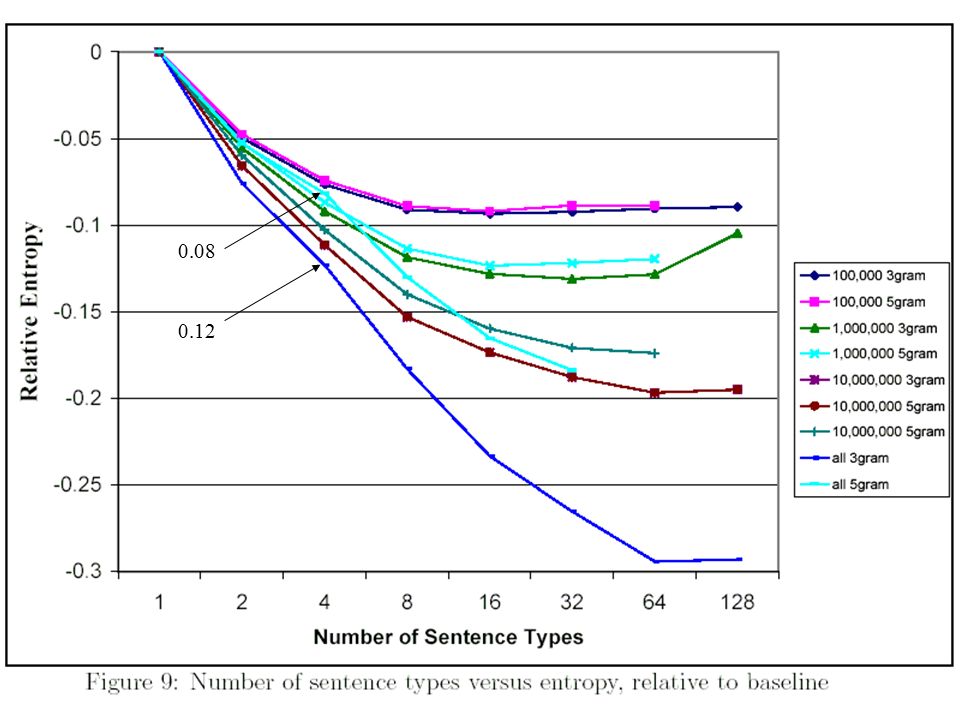
Relationship between training data size, n-gram order, and number of types

79
0.08 0.12
80
Sentence Mixture Models
Note that we don’t trust results for 128 mixtures. With 128 sentence types, there are 773 parameters, and the system may not have had enough heldout data to accurately estimate the parameters Ideally, we would run this experiment with a larger heldout set, but it already required 5.5 days with 20,000 words, so this is impractical

81
Sentence Mixture Models
We suspected that sentence mixture models would be more useful on larger training data size; with 100,000 words, only .1 bits, with 284,000,000 words, it’s nearly .3 bits This bodes well for the future of sentence mixture models : as computers get faster and larger, training data sizes should also increase

82
Sentence Mixture Models
Both 5-gram and sentence mixture models attempt to model long distance dependencies, the improvement from their combination would be less than the sum of the individual improvements In Fig.8, for 100,000 and 1,000,000 words, that different between trigram and 5-gram is very small, so the question is not very important For 10,000,000 words and all training data, there is some negative interaction 4 32 trigram 0.12 0.27 5-gram 0.08 0.18 So, approximately one third of the improvement seems to be correlated

83
Combining techniques Combining techniques interpolate this clustered trigram with a normal 5-gram :

84
Combining techniques Interpolate the sentence-specific 5-gram model with the global 5-gram model, the three skipping models, and the two cache model

85
Combining techniques Next, we define the analogous function for predicting words given clusters:

86
Combining techniques Now, we can write out our probability model : (9)
")
89
Experiment In fact, without KN-smooth, 5-gram actually hurt at small and medium data sizes. This is a wonderful example of synergy Caching is the largest gain at small and medium data size Combined with KN-smoothing, 5-grams are the largest gain at large data sizes

Similar presentations


 Slides are based on Introduction to Information Retrieval Book by Manning, Raghavan and Schütze.>")


 LING 570 Fei Xia Week 4: 10/21/2009 TexPoint fonts used in EMF. Read the TexPoint manual before you delete this box.: AAAAAA A A.>")


