Download presentation
Presentation is loading. Please wait.

1
The Discrete Fourier Transform

2
The Fourier Transform “The Fourier transform is a mathematical operation with many applications in physics and engineering that expresses a mathematical function of time as a function of frequency, known as its frequency spectrum.” – from http://en.wikipedia.org/wiki/Fourier_transform

3
The Fourier Transform “For instance, the transform of a musical chord made up of pure notes (without overtones) expressed as amplitude as a function of time, is a mathematical representation of the amplitudes and phases of the individual notes that make it up.” – from http://en.wikipedia.org/wiki/Fourier_transform
 expressed as amplitude as a function of time, is a mathematical representation of the amplitudes and phases of the individual notes that make it up. – from")
4
Amplitude & phase f(x) = sin( x + ) + – is the amplitude – is the frequency – is the phase – is the DC offset
 = sin( x + ) + – is the amplitude – is the frequency – is the phase – is the DC offset")
5
More generally f(x) = 1 sin( 1 x + 1 ) + 2 sin( 2 x + 2 ) +
 = 1 sin( 1 x + 1 ) + 2 sin( 2 x + 2 ) + ")
6
The Fourier Transform “The function of time is often called the time domain representation, and the frequency spectrum the frequency domain representation.” – from http://en.wikipedia.org/wiki/Fourier_transform

7
Applications differential equations geology image and signal processing optics quantum mechanics spectroscopy

8
REVIEW OF COMPLEX NUMBERS

9
Complex numbers Complex numbers... extend the 1D number line to the 2D plane are numbers that can be put into the rectangular form, a+bi where i 2 = -1, and a and b are real numbers.

10
Complex numbers (rectangular form)
")
11
Complex numbers Complex numbers... a is the real part; b is the imaginary part If a is 0, then a+bi is purely imaginary; if b is 0, then a+bi is a real number. originally called “fictitious” by Girolamo Cardano in the 16 th century

12
Complex arithmetic add/subtract – add/subtract the real and imaginary parts separately

13
Complex arithmetic complex conjugate – often denoted as – negate only the imaginary part

14
Complex arithmetic inverse where z is a complex number z bar is the length or magnitude of z a is the real part b is the imaginary part

15
Complex arithmetic multiplication (FOIL)
")
16
Complex arithmetic division complex conjugate of denominator

17
Complex numbers (polar form)
")
18
exponential vs. trigonometric Leonhard Euler 1707-1783 (phasor form)
")
19
DFT (DISCRETE FOURIER TRANSFORM)
")
20
DFT Say we have a sequence of N (possibly complex) numbers, x 0 … x N-1. The DFT produces a sequence of N (typically complex) numbers, X 0 … X N-1, via the following:
 numbers, X 0 … X N-1, via the following:.")
21
DFT & IDFT The DFT (Discrete Fourier Transform) produces a sequence of N (typically complex) numbers, X 0 … X N-1, via the following: The IDFT (Inverse DFT) is defined as follows:
 produces a sequence of N (typically complex) numbers, X 0 … X N-1, via the following: The IDFT (Inverse DFT) is defined as follows:")
22
Calculating the DFT So how can we actually calculate ?

23
Calculating the DFT So how can we calculate? Let’s use this relationship: Then So what does this mean?

24
Interpretation of DFT Back to the polar form: – r/N is the amplitude and is the phase of a sinusoid with frequency k/N into which x n is decomposed

25
CALCULATING THE DFT USING EXCEL

27
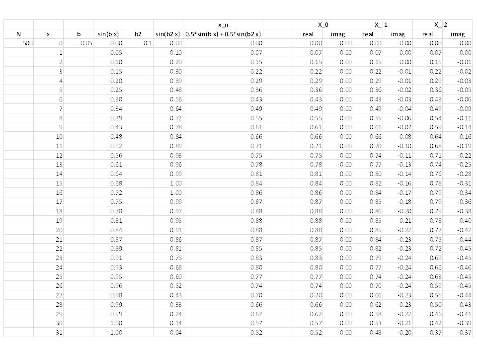
Check w/ matlab/octave % see http://www.mathworks.com/help/matla b/ref/fft.html http://www.mathworks.com/help/matla b/ref/fft.html N = 256;% # of samples n = (0:N-1);% subscripts b1 = 0.5;% freq 1 b2 = 2.5;% freq 2 xn = 0.5 * sin( b1*n ) + 0.2 * sin( b2*n ); plot( xn ); Xn = fft( xn ); plot( abs(Xn(1:N/2)) ); X0real= xn.* cos( -2*pi*n*0/N ); X0imag= xn.* sin ( -2*pi*n*0/N ); X1real= xn.* cos( -2*pi*n*1/N ); X1imag= xn.* sin ( -2*pi*n*1/N ); X2real= xn.* cos( -2*pi*n*2/N ); X2imag= xn.* sin ( -2*pi*n*2/N ); X3real= xn.* cos( -2*pi*n*3/N ); X3imag= xn.* sin ( -2*pi*n*3/N );. Note:.* is element-wise (rather than matrix) multiplication in matlab.
 multiplication in matlab..")
29
Add random noise. % see http://www.mathworks.com/help/matla b/ref/fft.html http://www.mathworks.com/help/matla b/ref/fft.html N = 256;% # of samples n = (0:N-1);% subscripts b1 = 0.5;% freq 1 b2 = 2.5;% freq 2 r = randn( 1, N );% noise xn = 0.5 * sin( b1*n ) + 0.2 * sin( b2*n ) + 0.5 * r; plot( xn ); Xn = fft( xn ); plot( abs(Xn(1:N/2)) ); X0real= xn.* cos( -2*pi*n*0/N ); X0imag= xn.* sin ( -2*pi*n*0/N ); X1real= xn.* cos( -2*pi*n*1/N ); X1imag= xn.* sin ( -2*pi*n*1/N ); X2real= xn.* cos( -2*pi*n*2/N ); X2imag= xn.* sin ( -2*pi*n*2/N ); X3real= xn.* cos( -2*pi*n*3/N ); X3imag= xn.* sin ( -2*pi*n*3/N );.
;% subscripts b1 = 0.5;% freq 1 b2 = 2.5;% freq 2 r = randn( 1, N );% noise xn = 0.5 * sin( b1*n ) * sin( b2*n ) * r; plot( xn ); Xn = fft( xn ); plot( abs(Xn(1:N/2)) ); X0real= xn.* cos( -2*pi*n*0/N ); X0imag= xn.* sin ( -2*pi*n*0/N ); X1real= xn.* cos( -2*pi*n*1/N ); X1imag= xn.* sin ( -2*pi*n*1/N ); X2real= xn.* cos( -2*pi*n*2/N ); X2imag= xn.* sin ( -2*pi*n*2/N ); X3real= xn.* cos( -2*pi*n*3/N ); X3imag= xn.* sin ( -2*pi*n*3/N );..")
30
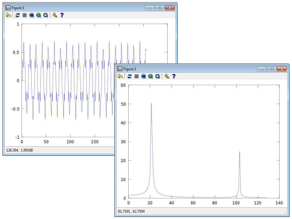
Signal without and with noise.

31
Signal with noise. FFT of noisy signal (two major components are still apparent).
.")
32
Example of differences in phase. xn = 0.5 * sin( b1*n ) + 0.2 * sin( b2*n ) xn = 0.5 * sin( b1*n – 0.5 ) + 0.2 * sin( b2*n )
 * sin( b2*n ) xn = 0.5 * sin( b1*n – 0.5 ) * sin( b2*n ).")
33
Computational complexity: DFT vs. FFT The DFT is O(N 2 ) complex multiplications. In 1965, Cooley (IBM) and Tukey (Princeton) described the FFT, a fast way (O(N log 2 N)) to compute the FT using digital computers. – It was later discovered that Gauss described this algorithm in 1805, and others had “discovered” it as well before Cooley and Tukey. – “With N = 106, for example, it is the difference between, roughly, 30 seconds of CPU time and 2 weeks of CPU time on a microsecond cycle time computer.” – from Numerical Recipes in C
 and Tukey (Princeton) described the FFT, a fast way (O(N log 2 N)) to compute the FT using digital computers. – It was later discovered that Gauss described this algorithm in 1805, and others had discovered it as well before Cooley and Tukey. – With N = 106, for example, it is the difference between, roughly, 30 seconds of CPU time and 2 weeks of CPU time on a microsecond cycle time computer. – from Numerical Recipes in C.")
34
Extending the DFT to 2D (and higher) Let f(x,y) be a 2D set of sampled points. Then the DFT of f is the following: (Note that engineers often use i for amps (current) so they use j for -1 instead.)
 so they use j for -1 instead.).")
35
Extending the DFT to 2D (and higher) In fact, the 2D DFT is separable so it can be decomposed into a sequence of 1D DFTs. And this can be generalized to higher and higher dimensions as well.

36
The classical “Gibbs phenomenon” Visit http://en.wikipedia.org/wiki/Square_wave. http://en.wikipedia.org/wiki/Square_wave Hear it at http://www.youtube.com/watch?v=uIuJTWS2 uvY. http://www.youtube.com/watch?v=uIuJTWS2 uvY

Similar presentations


 Algorithms Fast Fourier Transform (FFT) Algorithms.>")
,>")


>")


 Prof. Rob Stoll Department of Mechanical Engineering University of Utah Spring 2011.>")


; Phasors (7.3); Complex Numbers (Appendix) Prof. Phillips April 16, 2003.>")