1. DISCRETE FOURIER TRANSFORM
UNIT-I
DISCRETE FOURIER TRANSFORM

2. Syllabus Discrete Signals and Systems- A Review Introduction to DFT
Properties of DFT
Circular Convolution
Filtering methods based on DFT
FFT Algorithms
Decimation in time Algorithms,
Decimation in frequency Algorithms
Use of FFT in Linear Filtering.

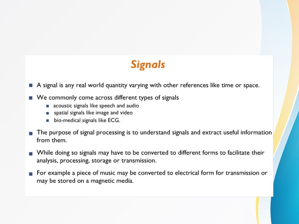
3. Signal Processing Humans are the most advanced signal processors
speech and pattern recognition, speech synthesis,…
We encounter many types of signals in various applications
Electrical signals: voltage, current, magnetic and electric fields,…
Mechanical signals: velocity, force, displacement,…
Acoustic signals: sound, vibration,…
Other signals: pressure, temperature,…
Most real-world signals are analog
They are continuous in time and amplitude
Convert to voltage or currents using sensors and transducers
Analog circuits process these signals using
Resistors, Capacitors, Inductors, Amplifiers,…
Analog signal processing examples
Audio processing in FM radios
Video processing in traditional TV sets

4. Limitations of Analog Signal Processing
Accuracy limitations due to
Component tolerances
Undesired nonlinearities
Limited repeatability due to
Tolerances
Changes in environmental conditions
Temperature
Vibration
Sensitivity to electrical noise
Limited dynamic range for voltage and currents
Inflexibility to changes
Difficulty of implementing certain operations
Nonlinear operations
Time-varying operations
Difficulty of storing information

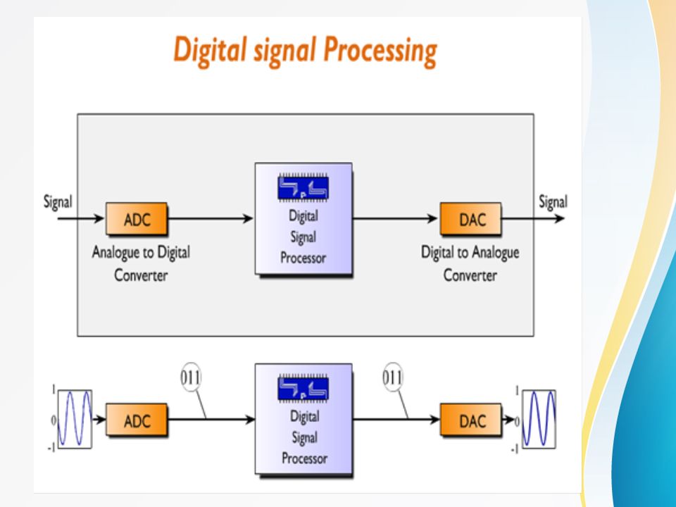
5. Digital Signal Processing
Represent signals by a sequence of numbers
Sampling or analog-to-digital conversions
Perform processing on these numbers with a digital processor
Digital signal processing
Reconstruct analog signal from processed numbers
Reconstruction or digital-to-analog conversion
A/D
DSP
D/A
analog
signal
digital signal
Analog input – analog output
Digital recording of music
Analog input – digital output
Touch tone phone dialing
Digital input – analog output
Text to speech
Digital input – digital output
Compression of a file on computer

7. Pros and Cons of Digital Signal Processing
Accuracy can be controlled by choosing word length
Repeatable
Sensitivity to electrical noise is minimal
Dynamic range can be controlled using floating point numbers
Flexibility can be achieved with software implementations
Non-linear and time-varying operations are easier to implement
Digital storage is cheap
Digital information can be encrypted for security
Price/performance and reduced time-to-market
Cons
Sampling causes loss of information
A/D and D/A requires mixed-signal hardware
Limited speed of processors
Quantization and round-off errors

8. Discrete Signals and Systems

12. Discrete-Time Signals: Sequences
Discrete-time signals are represented by sequence of numbers
The nth number in the sequence is represented with x[n]
Often times sequences are obtained by sampling of continuous-time signals
In this case x[n] is value of the analog signal at xc(nT)
Where T is the sampling period 20 40 60 80
100
-10 10
t (ms) 30 50
n (samples)

13. Basic Sequences and Operations
Delaying (Shifting) a sequence
Unit sample (impulse) sequence
Unit step sequence
Exponential sequences
-10 -5 5 10
0.5 1
1.5

14. Sinusoidal Sequences Important class of sequences
An exponential sequence with complex
x[n] is a sum of weighted sinusoids
Different from continuous-time, discrete-time sinusoids
Have ambiguity of 2k in frequency
Are not necessary periodic with 2/o

16. Discrete-Time Systems
Discrete-Time Sequence is a mathematical operation that maps a given input sequence x[n] into an output sequence y[n]
Example Discrete-Time Systems
Moving (Running) Average
Maximum
Ideal Delay System
x[n]
T{.}
y[n]

17. Memoryless System Memoryless System
A system is memoryless if the output y[n] at every value of n depends only on the input x[n] at the same value of n
Example Memoryless Systems
Square
Sign
Counter Example
Ideal Delay System

18. Linear Systems Linear System: A system is linear if and only if
Examples
Ideal Delay System

19. Time-Invariant Systems
Time-Invariant (shift-invariant) Systems
A time shift at the input causes corresponding time-shift at output
Example
Square
Counter Example
Compressor System

20. Causal System Causality Examples Counter Example
A system is causal it’s output is a function of only the current and previous samples
Examples
Backward Difference
Counter Example
Forward Difference

21. Stable System
Stability (in the sense of bounded-input bounded-output BIBO)
A system is stable if and only if every bounded input produces a bounded output
Example
Square
Counter Example
Log

22. DFS,DTFT & DFT

23. Fourier Transform of continuous time signals

24. Linear Time Invariant (LTI) Systems and z-Transform
If the system is LTI we compute the output with the convolution:
If the impulse response has a finite duration, the system is called FIR (Finite Impulse Response):

25. Z-Transform
Facts:
Frequency Response of a filter:

26. Frequency-Domain Properties
Time
Continuous
Discrete
Periodicity
Periodic
Aperiodic
Fourier Series
Continuous-Time
Fourier Transform
DFT
Duration
Finite
Infinite
Discrete-Time
and z-Transform
&
Periodic (2)
Discrete
&
Periodic

27. Signal Processing Methods
Periodicity
Periodic
Aperiodic
Fourier Series
Continuous-Time
Fourier Transform
Time
Continuous
Discrete
DFS
Discrete-Time
Fourier Transform
and z-Transform
Duration
Finite
Infinite

28. The Four Fourier Methods28

29. Relations Among Fourier Methods29

30. The Family of Fourier Transform
Aperiodic-Continuous－Fourier Transform

31. The Family of Fourier Transform
Periodic-Continuous－Fourier Series

32. The Family of Fourier Transform
Periodic-Discrete－DFS (DFT)

33. The Discrete Fourier Transform (DFT)
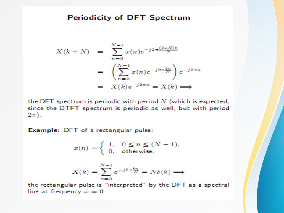
The DFS provided us a mechanism for numerically computing the discrete-time Fourier transform. But most of the signals in practice are not periodic. They are likely to be of finite length.
Theoretically, we can take care of this problem by defining a periodic signal whose primary shape is that of the finite length signal and then using the DFS on this periodic signal.
Practically, we define a new transform called the Discrete Fourier Transform, which is the primary period of the DFS.
This DFT is the ultimate numerically computable Fourier transform for arbitrary finite length sequences.
Introduction
为了计算有限长序列的傅氏变换，可定义一个周期性序列，有限长序列正好是该周期序列的一个周期，因此就可用DFS求其频谱。 33

34. The Discrete Fourier Transform (DFT)
Finite-length sequence & periodic sequence
Finite-length sequence that has N samples
periodic sequence with the period of N
Window operation
Periodic extension

35. The Family of Fourier Transform
Aperiodic-Discrete－DTFT

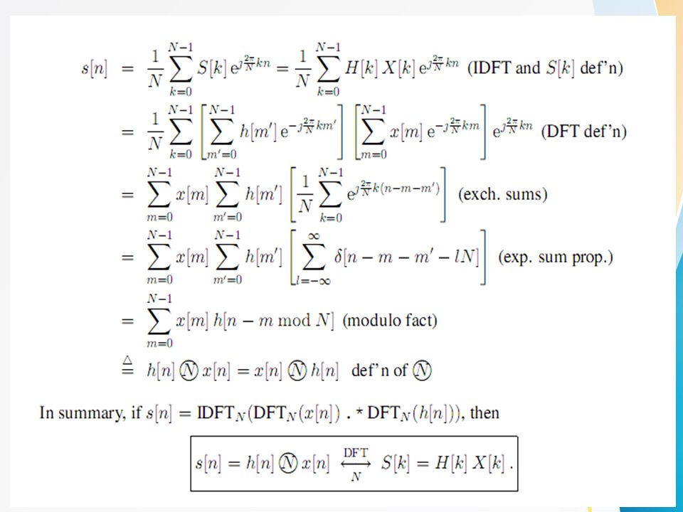
36. DFT and IDFT

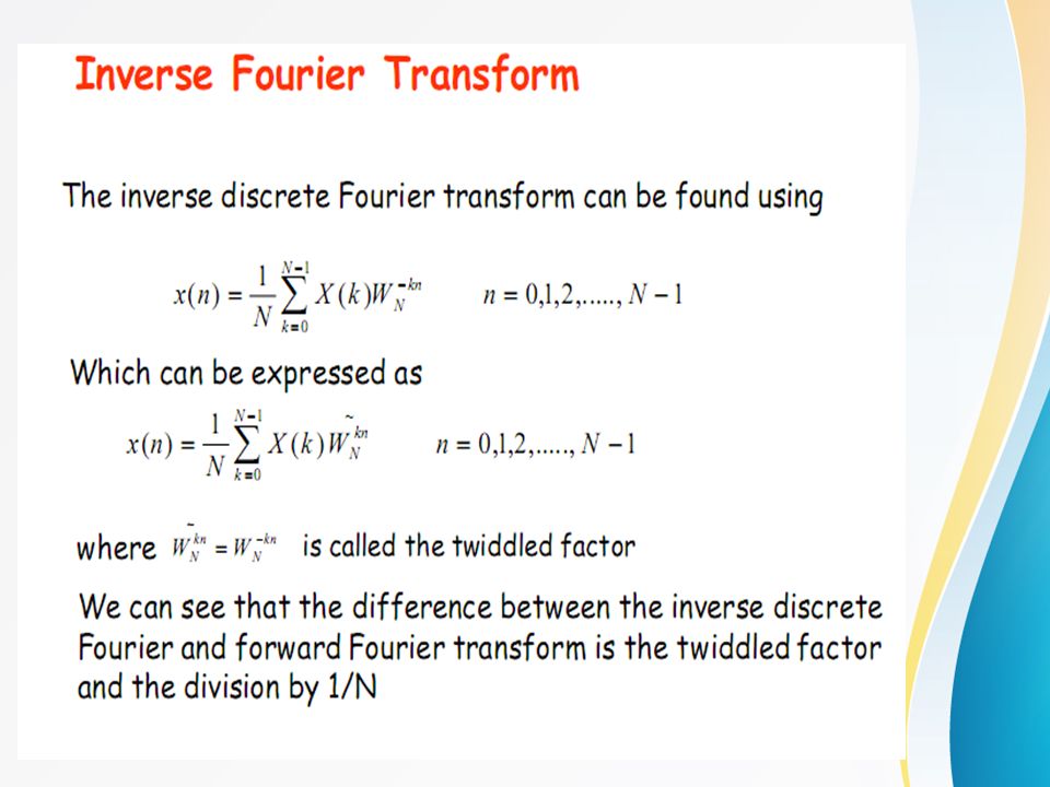
37. IDFT

38. The Discrete Fourier Transform (DFT)
The definition of DFT

39. Twiddle factor

40. Relationship of DFT to other transforms

42. Problems on DFT

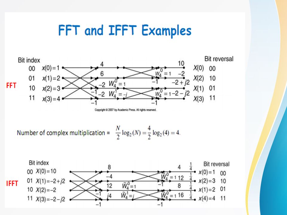
44. Example of DFT
Find X[k]
We know k=1,.., 7; N=8

45. Example of DFT

46. Example of DFT
Polar plot for
Time shift Property of DFT

47. Example of DFT

48. Example of DFT

49. Using the shift property!
Example of DFT
Summation for X[k]
Using the shift property!

50. Using the shift property!
Example of DFT
Summation for X[k]
Using the shift property!

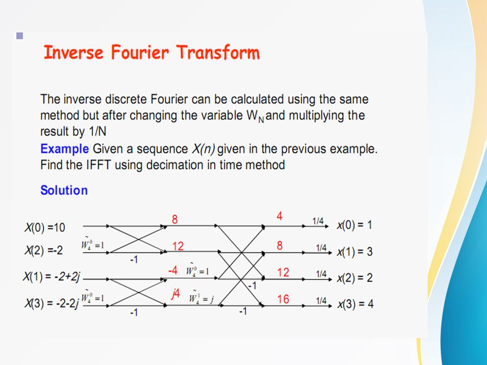
51. Example of IDFT
Remember:

52. Example of IDFT
Remember:

53. Problems on DFT

54. Problems on DFT

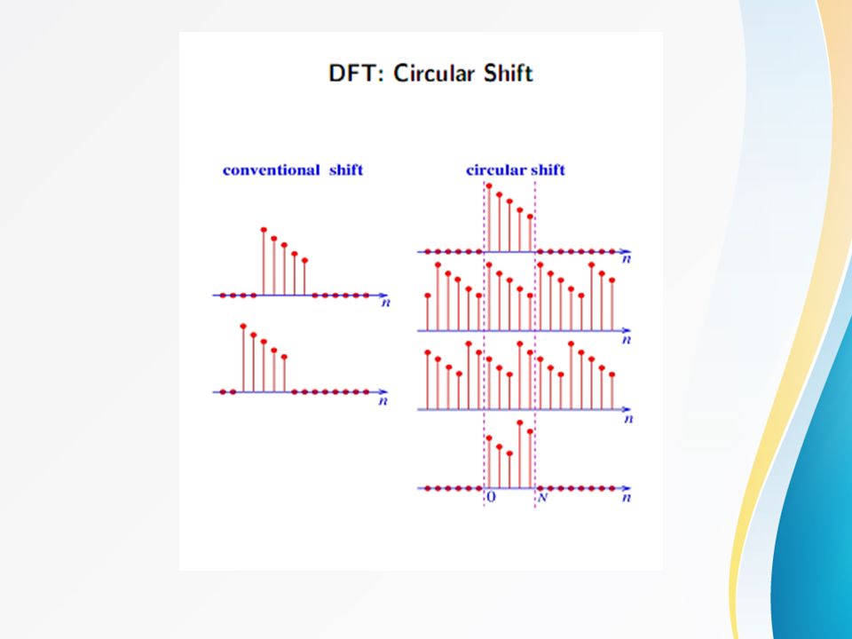
58. Circular shift of a sequence

62. The Properties of DFT Linearity Circular shift of a sequence
N3-point DFT, N3=max(N1,N2)
Circular shift of a sequence
Circular shift in the frequency domain

63. The Properties of DFT The sum of a sequence
The first sample of sequence

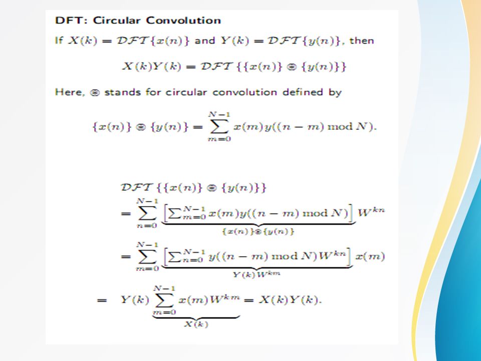
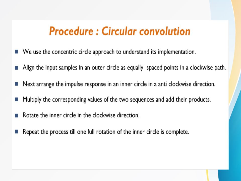
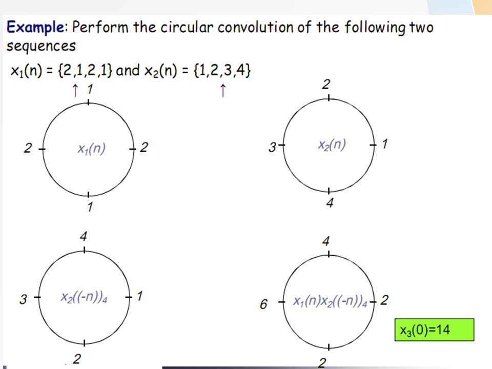
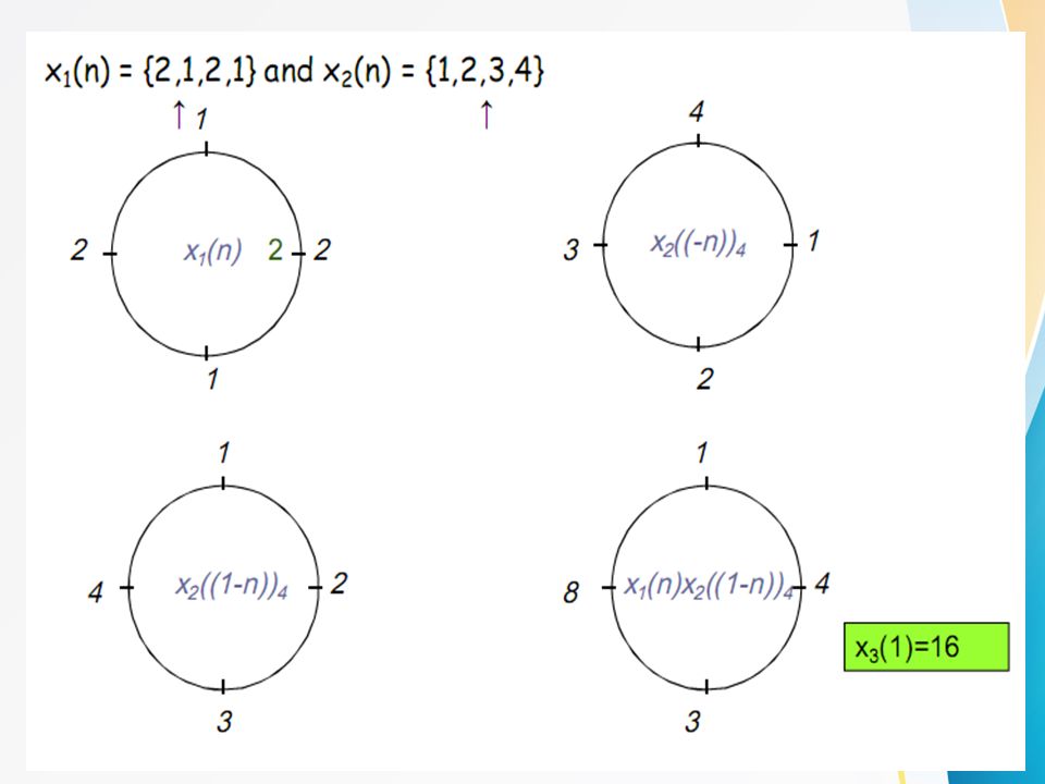
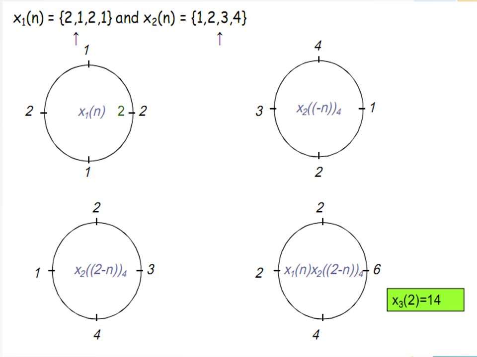
64. The Properties of DFT
Circular convolution N N N
Multiplication

65. The Properties of DFT
Circular convolution N N N
Multiplication

66. The Properties of DFT Circular correlation Linear correlation

67. The Properties of DFT

68. The Properties of DFT
Parseval’s theorem

69. The Properties of DFT Conjugate symmetry properties of DFT and
Let be a N-point sequence
x(-n)=x(N-n);
将x(n)看成是x~(n)的一个周期
在这里讲为何将x*(-n)的周期延拓写成x*((N-n))N期,主要从取模运算的方便性考虑
It can be proved that 69

70. The Properties of DFT Circular conjugate symmetric component
Circular conjugate antisymmetric
component

71. The Properties of DFT 71 对xep(n)的计算除了给出的画图方法之外，用直接计算的方法讲一遍。
举一个复数序列求圆周共轭对称分量的例子
x(n)={2+j1, 3+j2, 4-j3}, x*(n)={2-j1, 3-j2, 4+j3}
x*((N-n))NRN(n) ={2-j1, 4+j3,3-j2}
xep(n) ={2, 7/2+j5/2, 7/2-j5/2}
验证：xep*((N-n))NRN(n) ={2, 7/2+j5/2, 7/2-j5/2}=xep(n) 71

72. The Properties of DFT
and

73. The Properties of DFT 73 由Xep(k)和Xop(k)的定义即可得此公式
这里的偶对称指得是圆周偶对称。 73

74. The Properties of DFT Circular even sequences Circular odd sequences
实数偶对称－－实数偶对称
实数奇对称－－虚数奇对称 证明 74

75. Circular convolution in Time domain

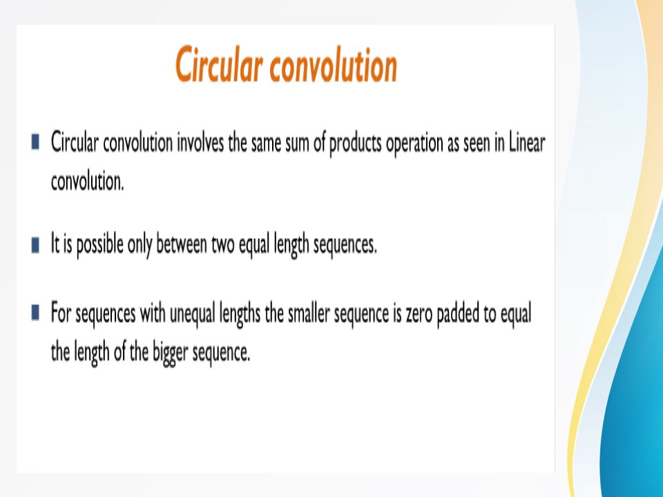
78. Circular convolution

84. Circular convolution-Example

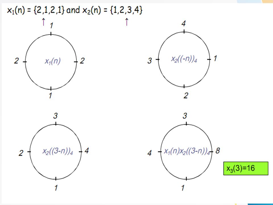
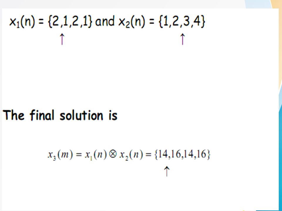
85. One sequence is distributed clockwise and
x1(n)=(1,2,3) and x2(n)=(4,5,6).
One sequence is distributed clockwise and
the other counterclockwise and the shift of the inner circle is clockwise. 1 1 * * 6 4 + + + +
= =28
= =31 4 5 5 6 * * * 3 2 * 3 2 + +
1st term
2st term 85

86. x1(n)* x2(n)=(1,2,3)*(4,5,6)=(18,31,31).
We have the same symmetry as before
3rd term 1 * 5 + +
=5+8+18=31 6 4 * * 3 2 + 86

87. Cirular convolution-Matrix method

88. Circular convolution property

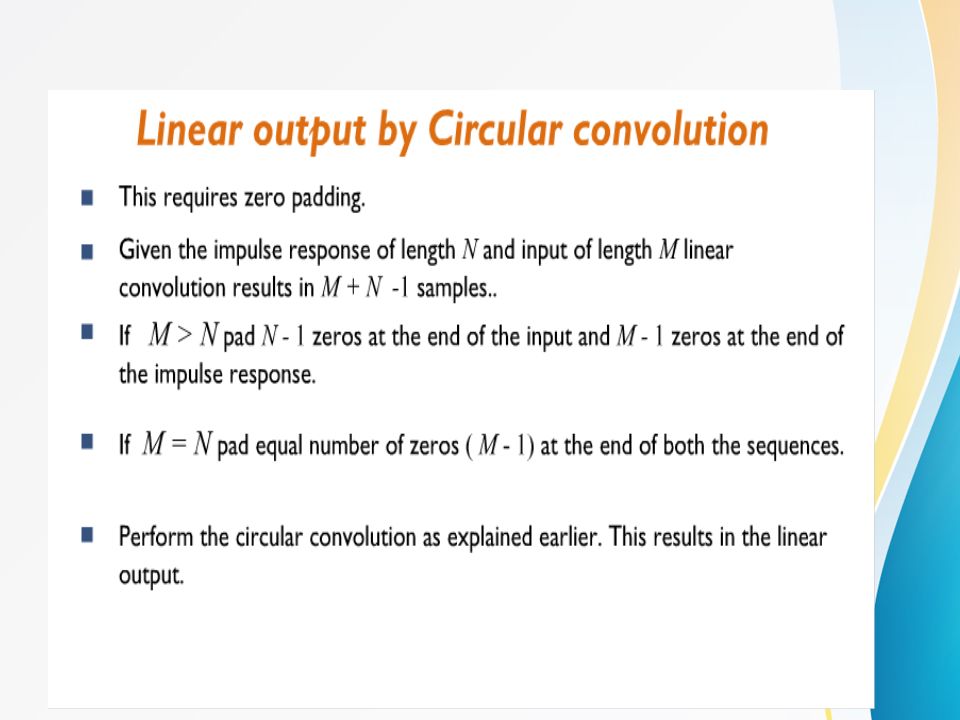
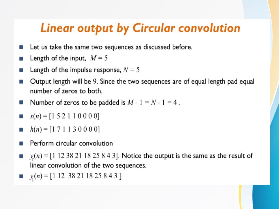
93. Use of DFT in linear filtering
DFT- based filtering always performs circular convolution.
But by zero padding adequetly,Circular convoltion can yield the same result.
where n=0.....(L+M-1)-1

94. Linear convolution using DFT

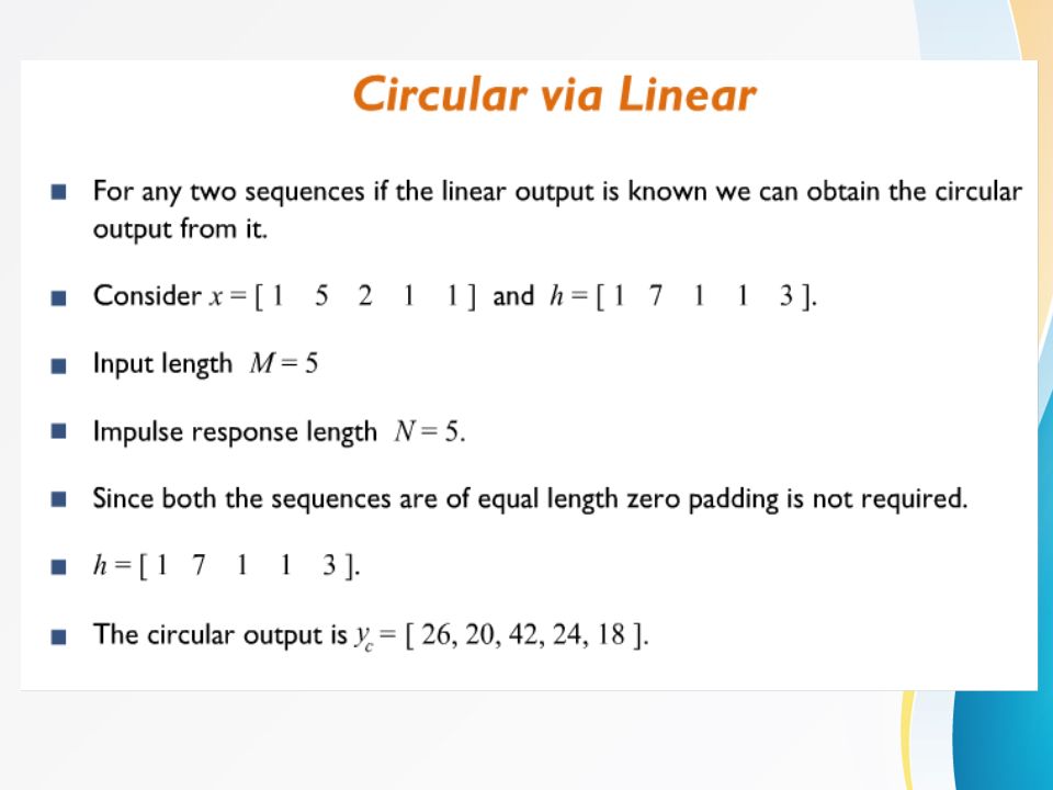
95. LINEAR & CIRCULAR CONVOLUTION
(1)calculate N point circular convolution by linear convolution
(2) calculate linear convolution by circular convolution
(3) calculate linear convolution by DFT

96. Example:Cir.conv

97. Circular conv

98. FAST FOURIER TRANSFORM

99. Discrete Fourier Transform
The DFT pair was given as
Baseline for computational complexity:
Each DFT coefficient requires
N complex multiplications
N-1 complex additions
All N DFT coefficients require
N2 complex multiplications
N(N-1) complex additions
Complexity in terms of real operations
4N2 real multiplications
2N(N-1) real additions
Most fast methods are based on symmetry properties
Conjugate symmetry
Periodicity in n and k

100. Properties-Example

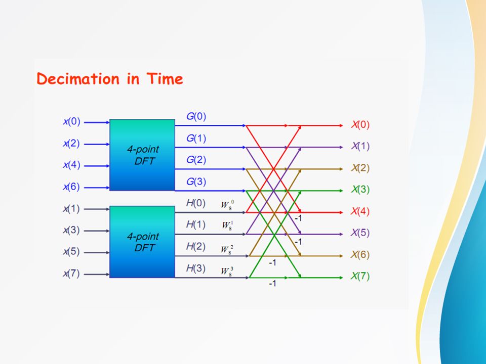
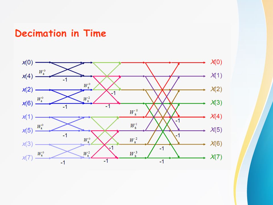
101. Decimation-In-Time FFT Algorithms
Makes use of both symmetry and periodicity
Consider special case of N an integer power of 2
Separate x[n] into two sequence of length N/2
Even indexed samples in the first sequence
Odd indexed samples in the other sequence
Substitute variables n=2r for n even and n=2r+1 for odd
G[k] and H[k] are the N/2-point DFT’s of each subsequence

102. Decimation In Time 8-point DFT example using decimation-in-time
Two N/2-point DFTs
2(N/2)2 complex multiplications
2(N/2)2 complex additions
Combining the DFT outputs
N complex multiplications
N complex additions
Total complexity
N2/2+N complex multiplications
N2/2+N complex additions
More efficient than direct DFT
Repeat same process
Divide N/2-point DFTs into
Two N/4-point DFTs
Combine outputs

104. DIT-FFT

107. Decimation In Time Cont’d
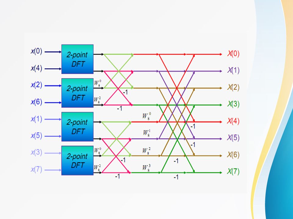
After two steps of decimation in time
Repeat until we’re left with two-point DFT’s

108. Decimation-In-Time FFT Algorithm
Final flow graph for 8-point decimation in time
Complexity:
Nlog2N complex multiplications and additions

109. Butterfly Computation
Flow graph constitutes of butterflies
We can implement each butterfly with one multiplication
Final complexity for decimation-in-time FFT
(N/2)log2N complex multiplications and additions

110. Decimation-in-time flow graphs require two sets of registers
In-Place Computation
Decimation-in-time flow graphs require two sets of registers
Input and output for each stage
Note the arrangement of the input indices
Bit reversed indexing

111. FFT Implementation Decimation in time FFT: Number of stages = log2N
Example: 8 point FFT
(1)Number of stages:
Nstages = 3
(2)Blocks/stage:
Stage 1: Nblocks = 4
Stage 2: Nblocks = 2
Stage 3: Nblocks = 1
(3)B’flies/block:
Stage 1: Nbtf = 1
Stage 2: Nbtf = 2
Stage 3: Nbtf = 2 W0 -1 W0 -1 W0 -1 W2 -1 W0 -1 W0 -1 W1 -1 W0 W0 -1 W2 -1 W0 -1 W2 -1 W3 -1
Decimation in time FFT:
Number of stages = log2N
Number of blocks/stage = N/2stage
Number of butterflies/block = 2stage-1

112. FFT Implementation Start Index Input Index 1 2 4 Twiddle Factor Index-1 W2 W1 W3
Stage 2
Stage 3
Stage 1
Start Index
Input Index 1 2 4
Twiddle Factor Index
N/2 = 4 4
/2 = 2 2
/2 = 1
Indicies Used W0 W2 W1 W3

113. Decimation-in-time FFT algorithm
Most conveniently illustrated by considering the special case of N an integer power of 2, i.e, N=2v.
Since N is an even integer, we can consider computing X[k] by separating x[n] into two (N/2)-point sequence consisting of the even numbered point in x[n] and the odd-numbered points in x[n].
or, with the substitution of variable n=2r for n even and n=2r+1 for n odd

114. That is, WN2 is the root of the equation WN/2=1 Consequently,
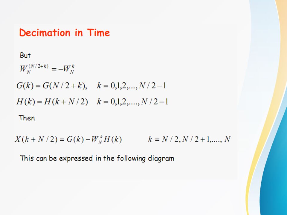
Since
That is, WN2 is the root of the equation WN/2=1
Consequently,
Both G[k] and H[k] can be computed by (N/2)-point DFT, where G[k] is the (N/2)-point DFT of the even numbered points of the original sequence and the second being the (N/2)-point DFT of the odd-numbered point of the original sequence.
Although the index ranges over N values, k = 0, 1, …, N-1, each of the sums must be computed only for k between 0 and (N/2)-1, since G[k] and H[k] are each periodic in k with period N/2.

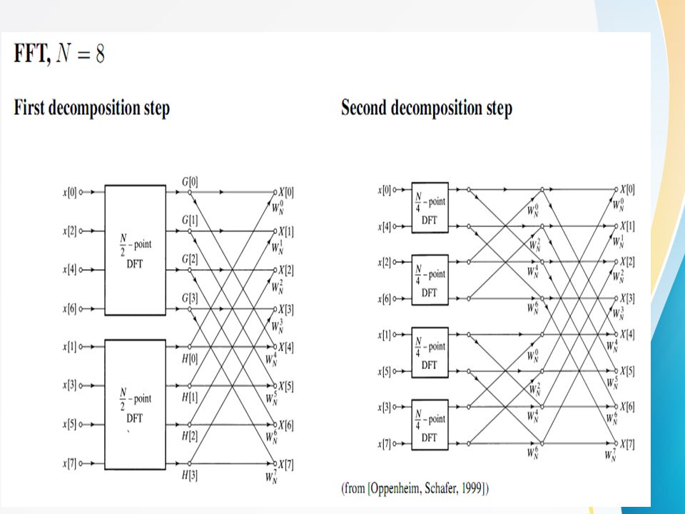
119. Decomposing N-point DFT into two (N/2)-point DFT for the case of N=8

120. We can further decompose the (N/2)-point DFT into two (N/4)-point DFTs
We can further decompose the (N/2)-point DFT into two (N/4)-point DFTs. For example, the upper half of the previous diagram can be decomposed as

121. Hence, the 8-point DFT can be obtained by the following diagram with four 2-point DFTs.

122. Finally, each 2-point DFT can be implemented by the following signal-flow graph, where no multiplications are needed.
Flow graph of a 2-point DFT

123. Flow graph of complete decimation-in-time decomposition of an 8-point DFT.

124. The butterfly computation can be simplified as follows:
In each stage of the decimation-in-time FFT algorithm, there are a basic structure called the butterfly computation:
The butterfly computation can be simplified as follows:
Flow graph of a basic butterfly computation in FFT.
Simplified butterfly computation.

125. Flow graph of 8-point FFT using the simplified butterfly computation

126. In the above, we have introduced the decimation-in-time algorithm of FFT.
Here, we assume that N is the power of 2. For N=2v, it requires v=log2N stages of computation.
The number of complex multiplications and additions required was N+N+…N = Nv = N log2N.
When N is not the power of 2, we can apply the same principle that were applied in the power-of-2 case when N is a composite integer. For example, if N=RQ, it is possible to express an N-point DFT as either the sum of R Q-point DFTs or as the sum of Q R-point DFTs.
In practice, by zero-padding a sequence into an N-point sequence with N=2v, we can choose the nearest power-of-two FFT algorithm for implementing a DFT.
The FFT algorithm of power-of-two is also called the Cooley-Tukey algorithm since it was first proposed by them.
For short-length sequence, Goertzel algorithm might be more efficient.

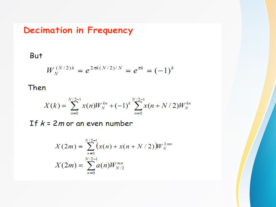
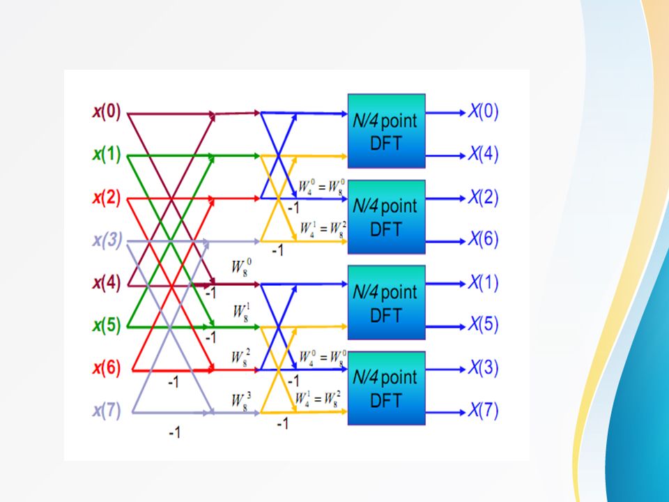
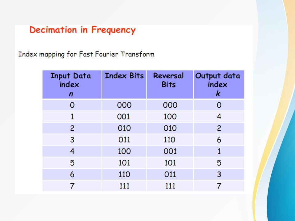
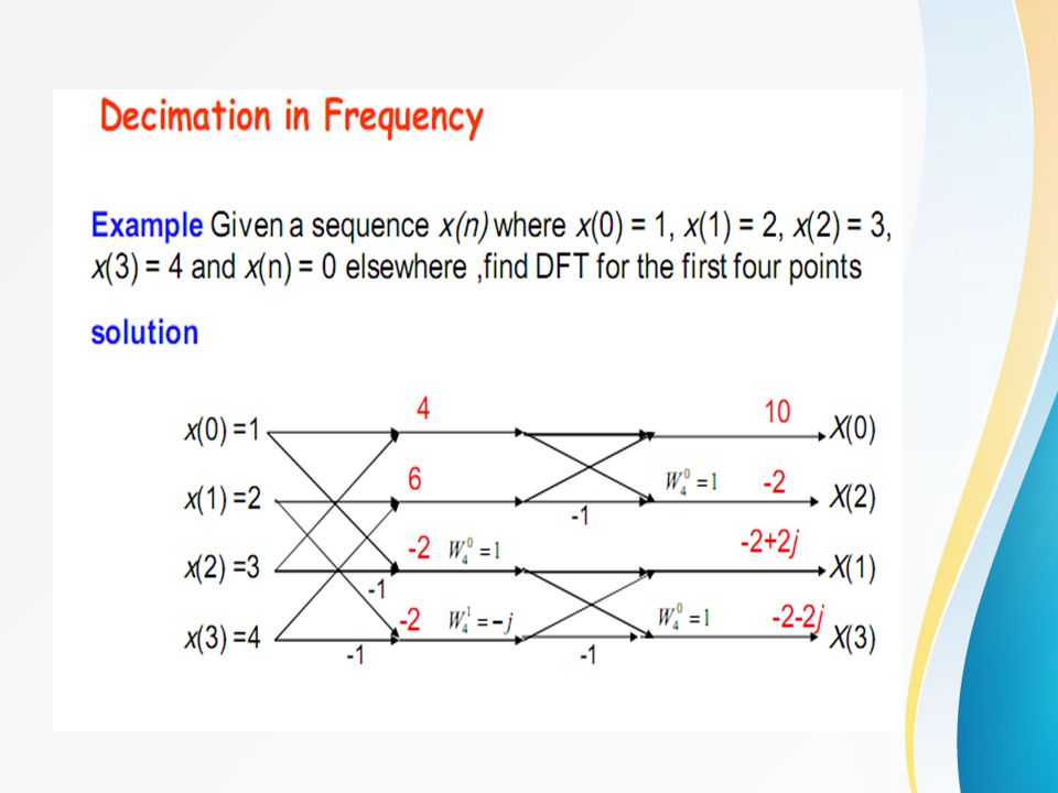
128. Decimation-In-Frequency FFT Algorithm
Final flow graph for 8-point decimation in frequency

129. Decimation-In-Frequency FFT Algorithm
The DFT equation
Split the DFT equation into even and odd frequency indexes
Substitute variables to get
Similarly for odd-numbered frequencies

131. Decimation in Frequency algorithm

132. Decimation in Frequency

134. DIF-FFT ALGORITHM

135. DIF-FFT ALGORITHM

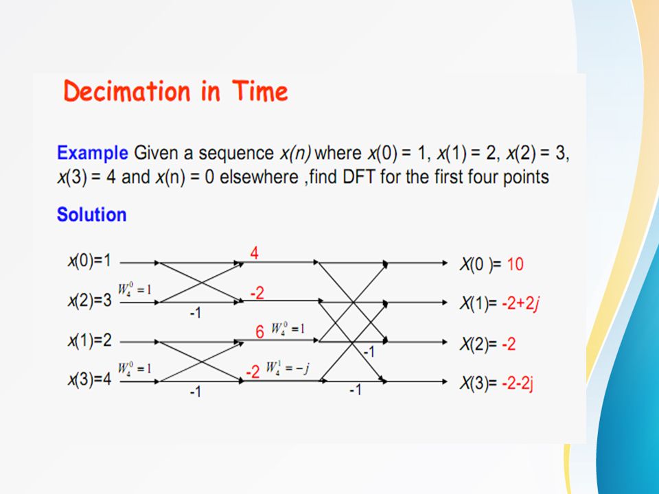
138. Example
Using decimation-in-time FFT algorithm compute DFT of the sequence
{-1 –1 –1 – }
Solution: Twiddle factors are

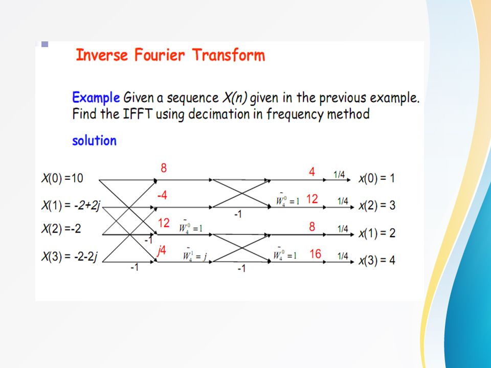
139. Solution and signal flow graph of the example

143. IDFT Using DIF-FFT