1. Chapter 5 .3 Riemann Sums and Definite Integrals

2. 5.3 The Area Problem
We want to find the area of the region S (shown on the next slide) that lies under the curve y = f(x) from a to b, where f is a continuous function with f(x) ≥ 0.
But what do we mean by “area”?
For regions with straight sides, this question is easy to answer:

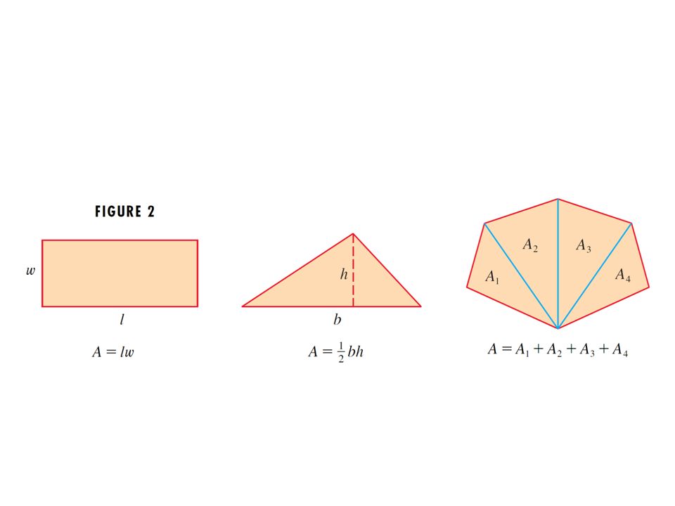
4. Area Problem (cont’d) For (see the figures on the next slide)…
a rectangle, the area is defined as length times width;
a triangle, the area is half the base times the height;
a polygon, the area is found by dividing the polygon into triangles and adding the areas.
But what if the region has curved sides?

6. Consider an object moving at a constant rate of 3 ft/sec.
Since rate . time = distance:
If we draw a graph of the velocity, the distance that the object travels is equal to the area under the line.
time
velocity
After 4 seconds, the object has gone 12 feet.

7. variable of integration
upper limit of integration
Integration
Symbol
integrand
variable of integration
(dummy variable)
lower limit of integration
It is called a dummy variable because the answer does not depend on the variable chosen.

8. If f(x) is continuous and non-negative on [a, b], then the definite integral represents the area of the region under the curve and above the x-axis between the vertical lines x = a and x = b

9. Area

10. Example:
Find the area under the curve from x=1 to x=2.
Area under the curve from x=1 to x=2.
Area from x=0
to x=2
Area from x=0
to x=1

11. Find the area between the x-axis and the curve from to .
Example:
Find the area between the
x-axis and the curve
from to
pos.
neg.

12. Note 2: is a number; it does not depend on x. In fact, we have
Note 3: The sum is usually called a Riemann sum.
Note 4: Geometric interpretations
For the special case where f(x)>0,
= the area under the graph of f from a to b.
In general, a definite integral can be interpreted as a difference of areas: x y o a b + -

13. Solution We compute the integral as the difference of the areas of the two triangles:y
y=x-1 A1 o A2 3 1 x -1

14. the rules for working with integrals, the most important of which are:1.
Reversing the limits changes the sign. 2.
If the upper and lower limits are equal, then the integral is zero. 3.
Constant multiples can be moved outside.

15. Reversing the limits changes the sign.1.
If the upper and lower limits are equal, then the integral is zero. 2.
Constant multiples can be moved outside. 3. 4.
Integrals can be added and subtracted.

16. 4.
Integrals can be added and subtracted. 5.
Intervals can be added
(or subtracted.)

17. 5.7 The Fundamental Theorem
If you were being sent to a desert island and could take only one equation with you,
might well be your choice.

18. The Fundamental Theorem of Calculus, Part 1
If f is continuous on , then the function
has a derivative at every point in , and

19. First Fundamental Theorem:
1. Derivative of an integral.

20. First Fundamental Theorem:
1. Derivative of an integral.
2. Derivative matches upper limit of integration.

21. First Fundamental Theorem:
1. Derivative of an integral.
2. Derivative matches upper limit of integration.
3. Lower limit of integration is a constant.

22. First Fundamental Theorem:
New variable.
1. Derivative of an integral.
2. Derivative matches upper limit of integration.
3. Lower limit of integration is a constant.

23. The long way:
First Fundamental Theorem:
1. Derivative of an integral.
2. Derivative matches upper limit of integration.
3. Lower limit of integration is a constant.

24. 1. Derivative of an integral.
2. Derivative matches upper limit of integration.
3. Lower limit of integration is a constant.

25. The upper limit of integration does not match the derivative, but we could use the chain rule.

26. The lower limit of integration is not a constant, but the upper limit is.
We can change the sign of the integral and reverse the limits.

27. We already know this! p The Fundamental Theorem of Calculus, Part 2
If f is continuous at every point of , and if F is any antiderivative of f on , then
(Also called the Integral Evaluation Theorem)
We already know this!
To evaluate an integral, take the anti-derivatives and subtract. p

28. The technique is a little different for definite integrals.
Example 10:
The technique is a little different for definite integrals.
new limit
We can find new limits, and then we don’t have to substitute back.
new limit
We could have substituted back and used the original limits.

29. Wrong! The limits don’t match! Example 8: Using the original limits:
Leave the limits out until you substitute back.
Wrong!
The limits don’t match!
This is usually more work than finding new limits

30. Example 9 as a definite integral:
No constants needed- just integrate using the power rule.
Rewrite in form of ∫undu

31. Substitution with definite integrals
Using a change in limits