1. Micro Data For Macro Models Topic 2: Consumption Inequality and Lifecycle Consumption

2. Part A: Background on Household Surveys (Jonathan Covered This in TA Sessions)

3. Micro Expenditure Data: Household Surveys Consumer Expenditure Survey (U.S. data) Starts in 1980 Broad consumption measures Some income and demographic data Repeated cross-sections Panel Study of Income Dynamics (U.S. data) Starts in late 60s Only food expenditure consistently Housing/utilities (most of the time) Broader measures (recently) Very good income and demographics Panel nature

4. Micro Expenditure Data: Household Surveys British Household Panel (British Data) oPanel data including income and expenditure Family Expenditure Survey (British Data) Bank of Italy Survey of Household Income and Wealth (Italian Data) oPanel data including income and expenditure There are others….many Scandinavian countries, Japan, Canada, etc. Even some developing economies have detailed household surveys that track some measures of consumption (e.g., Mexico, Taiwan, Thailand)

5. Micro Expenditure Data: Scanner Data Nielsen Homescan Data oLarge cross-section of households oVery detailed level transaction data (at the level of UPC code) oSome demographics oSome panel component oMatches quantities purchased with prices paid oCovers most of the large MSAs oMeasurement error? oSelection? oCoverage of goods?

6. Micro Income Data: Household Surveys Current Population Survey (CPS) oUsual data set used within U.S. to track labor supply and earnings. oHas panel component. oCan be found at www.ipums.org/cps/www.ipums.org/cps/ PSID Can be found at http://psidonline.isr.umich.edu/http://psidonline.isr.umich.edu/ Survey of Income and Program Participation (SIPP) oFour year rotating panel oLarge sample sizes oOver samples poor Census/American Community Survey oCan be found at www.ipums.orgwww.ipums.org

7. Part B: Trends in Consumption Inequality (Part 1)

8. 8 Income and Consumption Inequality Large literature documenting the increase in income inequality within the U.S. during the last 30 years (Katz and Autor, 1999; Autor, Katz, Kearney, 2008) Consumption is a better measure of well being than income (utility is U(C) not U(Y)). Does income inequality imply consumption inequality? Depends on whether income inequality is “permanent” Depends on insurance mechanisms available to households Depends on other margins of substitution (home production, female labor supply, etc.).

9. 9 Kevin Murphy’s Web Page

10. 10 Kevin Murphy’s Web Page

11. 11 Autor, Katz, Kearney (2008)

12. Why Do We Care About Consumption Inequality? Why is it important? oLearn about well being over time (economic growth, standard of livings, inequality, etc.). oLearn about insurance mechanisms available to households (public insurance, private insurance, etc.)? oLearn about the nature of income processes (more on this in the next set of lecture notes).

13. A Classic: Attanasio and Davis (1996)

14. A Short Discussion: The innovation of the Attanasio and Davis technique. The creation of synthetic cohorts from cross sectional data.

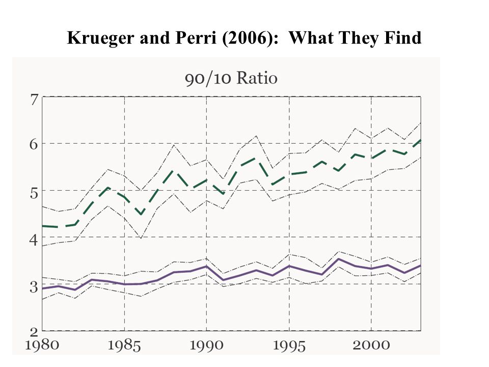
15. Krueger and Perri (2006) What they do: oUse data from the Consumer Expenditure Survey (CEX) to track the evolution of consumption inequality. oCEX is includes a nationally representative sample of households. -Designed to compute consumption weights for CPI -Short panel dimension (4 quarters) -Mostly used as repeated cross sections. -Includes detailed spending measures on expenditures by categories. oUse repeated cross sections to track consumption inequality.

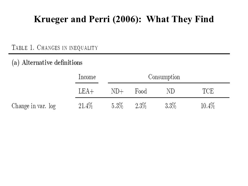
16. Krueger and Perri (2006): What They Find

19. Krueger and Perri (2005): What They Conclude Conclusions oIncome inequality is much greater than consumption inequality oIf some of the increase in income inequality is idiosyncratic, households can self insure (or public sector can provide insurance) making consumption inequality respond less than income inequality. oWrite down a model where insurance is endogenously provided. Increasing idiosyncratic shocks to income can increase demand for insurance (leading to more insurance). Consistent with their model, credit card access increased during this period. oBottom line: Use the consumption data to learn about the nature of income processes and insurance mechanisms.

20. Part C: A Caveat – Some Data Issues

21. 21 A Data Problem: Average Real Consumption in CEX

22. 22 A Data Problem: Average Real Consumption in CEX

23. 23 Percent Change in Consumption in CEX (from 1981)

24. 24 Trends in Real NIPA Aggregate Consumption

25. Part D: Revisiting Trends in Consumption Inequality Accounting for Measurement Error in Data

26. Can Measurement Error Alter Inequality Findings? Yes Depends on whether measurement error differs across the consumption (income) distribution. Suppose richer households have been underreporting their income to a greater extent in recent periods (relative to the past). The rich could be increasing their expenditure more (relative to other parts of the distribution). However, the systematic measurement error could also be increasing. How to test for group specific differences in measurement error?

27. Aguair and Bils (2011) Try to account for differential measurement error over different “income- demographic” groups to get a sense of changing consumption inequality. Some particulars: Define x ijt = average expenditure on good j, by group i, at time t j goods = food at home, clothing, utilities, entertainment, etc. i groups = cells based on income (5) and demographics (18) Define X it = average total expenditure for group i at time t. Formally:

28. Log budget share of good: ln w i = ln (x i /X ) Log total real expenditure: X = x Lux +x Normal +x Nec ln X 10 ln X 90 Estimated Engel curve for luxury Estimated Engel curve for normal good ln X 90 Observed 1980 Observed 2006 Inferred 2006 The Essence of the Exercise (From a Discussion by Jonathan Parker; NBER EFG 2011) Inferred adjustment to ln X 90 ln X 10

29. Aguair and Bils (2011) Assume measurement error in expenditure…… represents a good specific error (common across all groups) represents a group specific error (common across all goods)

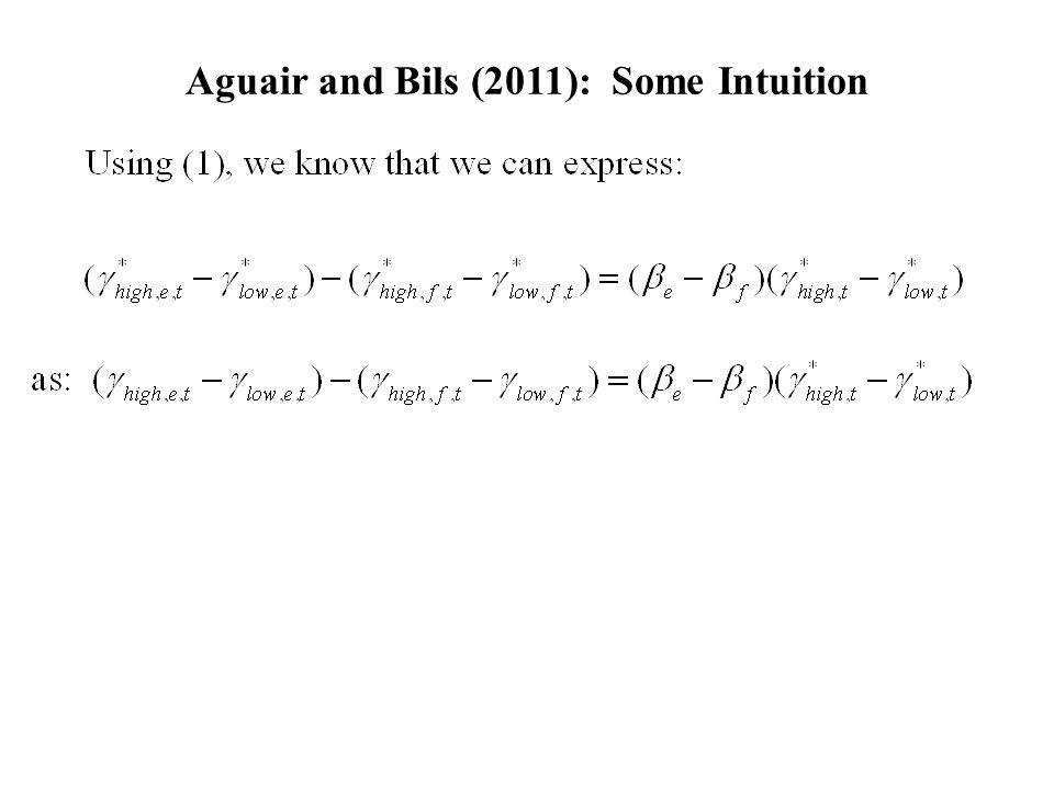
30. Aguair and Bils (2011): Some Intuition Difference-in-Difference Estimates (2 good case, 2 group case) Goods = e (entertainment) and f(food) Groups = high (rich) and low (poor) (difference out good specific error)

31. Aguair and Bils (2011): Some Intuition Take differences across goods to eliminate group specific error Obtain an unbiased estimate of relative consumption inequality. Need to map into units of total expenditure. Want to recover:

32. Aguair and Bils (2011): Some Intuition

34. Aguair and Bils (2011) Suppose for true expenditures, x * : Can estimate the following using actual data in some period 0 where systematic measurement error is less of an issue: If there is no measurement error in the data, can uncover: Assumes income elasticities are constant over time (and can be locally estimated). Assume measurement error is zero in period 0.

35. Aguair and Bils (2011): Some Intuition Substituting in the estimated β’s, we get:

36. 36 Aguiar and Bils (2011) Findings

37. 37 Aguiar and Bils (2011) Findings

38. 38 Aguiar and Bils (2011) Findings Relative Spending Differences Between High and Low Income Groups

39. 39 Aguiar and Bils (2011) Findings

40. 40 Aguiar and Bils (2011) Findings Different Saving Rates From the CEX

41. Attanasio, Hurst, and Pistaferri (2012) Also show that measurement error likely results in the underestimation of changes in consumption inequality within the U.S. Like Aguiar and Bils, find that consumption inequality and income inequality have moved essentially one-for-one over the past thirty years. Use other empirical approaches and data sets. You can find a copy of the paper on my web page (under working papers).

42. Attanasio, Hurst, and Pistaferri (2012) Use CE Diary Data (a separate survey) as opposed to CE Interview Data (which was used by Krueger/Perri and Aguiar/Bils. Diary data found to have less measurement error (better matches NIPA trends).

43. Attanasio, Hurst, and Pistaferri (2012) Imputed PSID Consumption matches income inequality nearly identically. Food PSID Consumption also matches income inequality trends (need to scale by food income elasticity which is about 0.5).

44. Conclusions: Part 1 (A – D) Measurement error is important in Consumer Expenditure Survey! Even though there is measurement error, can still measure consumption inequality. Without controlling for measurement error, looks like small increases in consumption inequality. Much of that is due to the rich reporting less and less of their expenditures. Controlling for the systematic recent underreporting of the rich increases the estimated consumption inequality in the U.S. to levels that match the changing income inequality.

45. Part E: Overview of Lifecycle Expenditures

46. Why Do We Care About Lifecycle Expenditure? Why is it important? -Learn about household preferences broadly C.E.S. vs. log vs. other / Habits? / Status? -Estimate preference parameters intertemporal elasticity of substitution/ risk aversion/ discount rate -Learn about income process permanent vs. transitory shocks / expected vs. unexpected -Learn about financial markets/constraints liquidity constraints / risk sharing arrangements -Learn about policy responses spending after tax rebates, fiscal multipliers, etc.

47. Why Do We Care (continued)? The big picture with consumption: -Use estimated parameters to calibrate models -Understand business cycle volatility -Conduct policy experiments (social security reform, health care reform, tax reform, etc.) -Estimate responsiveness to fiscal or monetary policy -Broadly understand household behavior

48. How We Will Proceed The outline of the next part of the lecture: -Understand lifecycle consumption movements oIllustrative of how one fact can spawn multiple theories. oShow how a little more data can refine the theories oIllustrate the empirical importance of the Beckerian consumption model (i.e, incorporating home production and leisure).

49. Fact 1: Lifecycle Expenditures Plot: Adjusted for cohort and family size fixed effects

50. Define Non-Durable Consumption (70% of outlays) Use a measure of non-durable consumption + housing services Non-durable consumption includes: Food (food away + food at home)Entertainment Services Alcohol and TobaccoUtilities Non-Durable TransportationCharitable Giving Clothing and Personal CareNet Gambling Receipts Domestic ServicesAirfare Housing services are computed as: Actual Rent (for renters) Imputed Rent (for home owners) – Impute rent two ways Exclude: Education (2%), Health (6%), Non Housing Durables (16%), and Other (5%) >

51. Empirical Strategy: Lifecycle Profile of Expenditure Estimate: (1) where is real expenditure on category k by household i in year t. Note: All expenditures deflated by corresponding product-level NIPA deflators. Cohort it = year-of-birth (5 year range – i.e., 1926-1930) D t = Vector of normalized year dummies (See Hall (1968)) Family Composition Controls: Household size dummies, Number of Children Dummies Marital status dummies, Detailed Age of Children Dummies

52. Fact 2: Hump Shaped Profile – By Education From Attanasio and Weber (2009)

53. Fact 3: Retirement Consumption Dynamics From Bernheim, Skinner and Weinberg (AER 2001)

54. The Puzzle? (Friedman, Modigliani, Hall, etc.) {N t, V t } are permanent and transitory mean zero shocks to income with underlying variances equal to σ 2 N and σ 2 V

55. Preferences

56. Euler Equation

57. What Are Potential Taste Shifters Over Life Cycle 1.Family Size oMakes some difference oHump shaped pattern still persists oSee Facts 1 and 3 (above) – these were estimated taking out detailed family size controls. 2.Other Taste Shifters (that change over the lifecycle – for a given individual)?

58. 58 Fact 4: Deaton and Paxson (1994) “Intertemporal Choice and Inequality” (JPE) Hypotheses: PIH implies that for any cohort of people born at the same time, inequality in both consumption and income should grow with age. How much consumption inequality grows informs researchers about: o Lifecycle shocks to permanent income o Insurance mechanisms available to households. Data:U.S., Great Britain, and Taiwan

59. 59 Deaton and Paxson Methodology (U.S. Application) Variance of Residual Variation Compute variance of ε k it at each age and cohort Regress variance of ε k it on age and cohort dummies Plot age coefficients (deviation from 25 year olds) Note: This is my application of the Deaton/Paxson Methodology (very similar in spirit to theirs).

60. Fact 4: Deaton-Paxson Cross Sectional Dispersion: With and With Out Housing Services

61. Cross Sectional Variance of Total Nondurables for 25 Year Olds = 0.16

62. Fact 4: Deaton-Paxson Cross Sectional Dispersion: With and With Out Housing Services Cross Sectional Variance of Total Nondurables for 25 Year Olds = 0.16

63. Questions: 1.What Else Drives the Hump Shaped Expenditure Profile? 2.Why Does Expenditures (on food) Fall Sharply At Retirement? 3.Why Does Cross Sectional Consumption Inequality Increase Over the Lifecycle?

64. Explanations for Questions (1) and/or (2) Liquidity Constraints and Impatience - Gourinchas and Parker (2002) Myopia - Keynes (and others) Time Inconsistent Preferences (with liquidity constraints) - Angeletos et al (2001) Habits and Impatience Non-Separable Preferences Between Consumption and Leisure - Heckman (1974) Home Production/Work Related Expenses - Aguiar and Hurst (2005, 2008)

65. Part F: Gourinchas and Parker (2002)

66. Gourinchas and Parker (2002) “Consumption Over the Lifecycle” (Econometrica) You should read this paper. Estimates lifecycle consumption profiles in the presence of realistic labor income uncertainty (via calibration). Use CEX data on consumption (synthetic cohorts). Estimates the riskiness of income profiles (from the Panel Study of Income Dynamics) and feeds those into the model. Use the model and the observed pattern of lifecycle profiles of expenditure to estimate preference parameters (risk aversion and the discount rate).

67. Gourinchas and Parker Structure Impose some liquidity constraints on model: W t > some exogenous level

68. Goal of Gourinchas-Parker: Estimate Utility Parameters Intertemporal elasticity of substitution (I.E.S.) (1/ρ) Risk Aversion (ρ) Time Discount Factor (β = 1/(1+ δ)) Note:Risk aversion = (1/I.E.S.) with CES preferences

69. Why is the I.E.S. (1/ρ) important? The intertemporal elasticity of substitution determines how levels of consumption respond over time to changes in the price of consumption over time (which is the real interest rate – or more broadly – the real return on assets). This parameter is important for many macro applications. Economics: Raising interest rates lowers consumption today (substitution effect) Raising interest rates raises consumption today (income effect – if net saver) Consumption tomorrow unambiguously rises

70. Graphical Illustration – No Substitution Effect 1 2 period C Low interest rate High interest rate ΔC 2 = X ΔC 1 = X With only an income effect – consumption growth rate will not respond to interest rate changes. Estimate of (1/ρ) = 0.

71. Graphical Illustration – With Substitution Effect 1 2 period C Low interest rate High interest rate ΔC 2 > X ΔC 1 < X As the substitution effect gets stronger, the growth rate of consumption increases more as interest rates increase. Estimate of (1/ρ) > 0.

72. One Way to Estimate I.E.S.

73. Issues With Estimating I.E.S. Use of data source (micro or aggregate) Forecast of future interest rates? Correlation of forecast of interest rate with error term (things that make interest rates go up could be news about permanent income – which affect consumption). Hall (1988) “Intertemporal Substitution in Consumption” (JPE; 1/ρ = 0) Attanasio and Weber (1993) “Consumption Growth, the Interest Rate and Aggregation” (ReStud; 1/ρ = 0.60-0.75). Vissing-Jorgensen (2002) “Limited Asset Market Participation and the Elasticity of Intertemporal Substitution” (JPE; 1/ρ = 0.3 (stockholders) and 1/ρ = 0.8 (bondholder).

74. Gournichas-Parker Methodology: Calibration Choose preference parameters that match the lifecycle profiles of consumption given the mean and variance of income process. Use synthetic individuals (based on education and occupation) Using PSID Computed “G” from the data (mean growth rate of income over the lifecycle). Estimated the variances from the data. Using CEX Compute lifecycle profiles of consumption Compute lifecycle profile of wealth/income (at beginning of life)

75. Intuition No Uncertainty: No “Buffer Stock Behavior” (uncertainty coupled with liquidity constraints) Consumption growth determined by Rβ (where β = 1/(1+δ)) With Income Uncertainty Buffer stock behavior takes place (household reduce consumption and increase saving to insure against future income shocks). Consumption will track income if households are sufficiently “impatient” Sufficiently Impatient with Uncertainty: RβE[(GN) -ρ ] < 1

76. Results Estimates (Base Specification): δ= 4.2% - 4.7% (higher than chosen r = 3.6%) ρ= 0.5 – 1.4(1/ρ = 0.6 – 2.0) Interpretation Early in the lifecycle, households act as “buffer stock households”. As income growth is “high”, consumption tracks income (do not want to accumulate too much debt to smooth consumption because of income risk) In the later part of the lifecycle, consumption falls because households are sufficiently impatient such that δ > r.

77. Gourinchas-Parker Conclusions Optimizing model of household behavior with income risk can match the lifecycle profile of household consumption Liquidity constraints can explain early life patterns. Impatience explains the late lifecycle patterns. Households face significant labor earnings risk (holding assets early in lifecycle even though they are impatient). Take Away:Households are sufficiently impatient Households face non-trivial income risk (even in middle age).

78. Part G: The Beckerian Model of Consumption

79. Ghez and Becker (1975); Aguiar, Hurst and Karabarbounis (2011) subject to: Let μ, λ, θ, and κ be the respective multipliers on the time budget constraint, the money budget constraint, the positive hours constraint and the positive assets constraint. Assume U(.) is additively separable across time and across goods. ψ= is vector of wages, commodity prices (p), taxes and transfers ( assume C.E.S., CRS)

80. First Order Conditions If θ = 0 (L > 0), price of time (in permanent income units) (μ/λ = w) More generally (given L often = 0), μ/λ = ω

81. First Order Conditions Intra-period tradeoff between time and goods: (1) Marginal rate of transformation between time and goods in production of n is equated to the relative price of time.

82. First Order Conditions A few assumptions: oF i is constant elasticity of substitution op i ’s are constant over time Some algebra (2) (3) Note: To get (3), sub (2) into (1)

83. Static First Order Condition The static F.O.C. pins down expenditure relative to time inputs. If we know σ and the change in the opportunity cost of time, we should be able to pin down the relative movement in expenditures relative to time. %ΔX i -%ΔH i =σ i %Δω Notice, this equation does not require us to make any assumptions about borrowing or lending, perfect foresight, etc.

84. More Intuition (Assume separability in c n ’s) Differentiate FOC for x n with respect to ω holding λ constant. Get: This is just Ghez and Becker (1975) Need to compare the intra-elasticity of substitution between time and goods (σ) to the elasticity of substitution in utility across consumption goods (γ). Note:Complicates mapping of expenditures into permanent income in general and the estimation of Engel curves in particular.

85. Different Than Standard Predictions Differentiate FOC for x n with respect to ω holding λ constant. Get: Spending should fall the most (with declines in the marginal value of wealth) for goods that have high elasticities of substitution (high income elasticities).

86. Implications For given resources (λ): – As the price of time increases, consumers substitute market goods for time (X i increases) – depends on σ i – As the price of time increases, consumers substitute to goods (periods) in which consumption is “cheaper” (X i falls) – depends on γ i What goods have high/low σ: -High σ: goods for which home production is an available margin of substitution (e.g., food) -Low σ: goods for which time and spending are complements (e.g., entertainment goods) What goods have high/low γ: -High γ: goods which have a high income elasticity (luxuries) -Low γ:goods which have a low income elasticity (necessities)

87. Predictions: Lifecycle Movements Gourinchas and Parker model (and most other models) oLuxuries (entertainment) should decline more late in life relative to necessities (food) oNo importance of changing opportunity cost of time over lifecycle Beckerian Model oGoods for which home production is important can move over the lifecycle in ways that are different than goods for which expenditure and time are complements. oIf opportunity cost of time declines after middle age, food may decline more than entertainment later in life.

88. Part H: Tests for Beckerian Model of Consumption

89. Test 1: Aguiar and Hurst “Consumption vs. Expenditure” (JPE 2005)

90. 90 Question What causes the decline in spending for households at the time of retirement? Bernheim, Skinner, and Weinberg (AER 2001) “What Accounts for the Variation in Retirement Wealth Among U.S. Households” oPeople do not plan for retirement (myopic) Banks, Blundell, and Tanner (AER 1998) “Is There a Retirement Savings Puzzle” oPeople get bad news (on average) at retirement (shock to λ) Hundreds of other papers documenting similar patterns for different countries. Do not think about the cost of time changing with retirement.

91. Fact 3: Retirement Consumption Dynamics From Bernheim, Skinner and Weinberg (AER 2001)

92. 92 Our Approach: Measuring Consumption Directly Main Data Set: Continuing Survey of Food Intake of Individuals (CSFII) – Conducted by Department of Agriculture – Cross Sectional / Household Level Survey – Two recent waves: Wave 1 (1989 -1991) ; Wave 2 (1994-1996) – Nationally Representative – Multi Day Interview – All individuals within the household are interviewed (C at individual level) – Tracks final food intake (not intermediate goods --- think about a cake) Detailed food expenditure, demographic, earnings, employment, and health measures Large sample sizes: –6,700 households in CSFII-91 –8,100 households in CSFII-96 Focus on intake NOT expenditure!

93. 93 Actual Consumption Data (CSFII) The key to the data: 24 hour food intake diaries (asked for all days in the survey) Diaries are detailed: –Amount of food item consumed (detailed 8 digit food codes) –Brand of food item (often unusable by researchers) –Cooking method –Condiments added Dept of Agriculture converts the total day’s food intake into several nutritional measures (calories, protein, saturated fat, total fat, vitamin C, riboflavin, etc.). –The conversion is made using all food diary data (i.e., brand, whether cooked with butter).

94. 94 8 digit food codes: Cheese Example 18 of the 100 8-digit codes for cheese. 14101010 CHEESE, BLUE OR ROQUEFORT 14102010 CHEESE, BRICK 14102110 CHEESE, BRICK, W/ SALAMI 14103020 CHEESE, BRIE 14104010 CHEESE, NATURAL, CHEDDAR OR AMERICAN TYPE 14104020 CHEESE, CHEDDAR OR AMERICAN TYPE, DRY, GRATED 14104200 CHEESE, COLBY 14104250 CHEESE, COLBY JACK 14105010 CHEESE, GOUDA OR EDAM 14105200 CHEESE, GRUYERE 14106010 CHEESE, LIMBURGER 14106200 CHEESE, MONTEREY 14106500 CHEESE, MONTEREY, LOWFAT 14107010 CHEESE, MOZZARELLA, NFS (INCLUDE PIZZA CHEESE) 14107020 CHEESE, MOZZARELLA, WHOLE MILK 14107030 CHEESE, MOZZARELLA, PART SKIM (INCL ""LOWFAT"") 14107040 CHEESE, MOZZARELLA, LOW SODIUM 14107060 CHEESE, MOZZARELLA, NONFAT OR FAT FREE

95. 95 Changes in “Spending” At Retirement Run: ln(x i ) = γ 0 + γ 1 Retired i + γ 2 Z i + error i Retired i is a dummy variable equal to 1 if the household head is retired. Instrument Retired i status with age dummies (potential endogeneity) Z includes: race, sex, health, region, time, family structure controls Sample: Relatively “young” older households: Heads aged 57-71 Total food expenditure (x) falls by 17% for retired households (γ 1 ), p-value < 0.01 Other results: –Food expenditure at home falls by 15% –Food expenditure away from home falls by 31%

96. 96 Changes in “Consumption” at Retirement How do we turn these food diaries into meaningful measures of consumption? Our approach: 1. Examine Nutritional Quality of Diet (vitamins, cholesterol, fat, calories, etc.) 2.Examine individual goods with strong income elasticities (hotdogs, fruit, yogurt, shellfish, wine) 3.Luxury/Quality goods (e.g. brands vs generics, lean vs. fatty meat) 4. Use structural model to aggregate food consumption data and perform formal PIH test.

97. 97 Nutritional Measures Regress: ln(c i ) = α 0 + α 1 ln(y perm ) + demographics > Regress: ln(c i ) = β 0 + β 1 Retired + demographics > Consumption Measure (in logs) Estimated Elasticity (α 1 ) Retirement Effect (β 1 ) Calories -4% (2%) -2% (4%) Protein * -1% (1%) -3% (2%) Vitamin A * 44% (5%) 36% (9%) Vitamin C * 34% (5%) 33% (9%) Vitamin E * 18% (3%) 11% (4%) Calcium* 10% (2%) 13% (4%) Cholesterol * - 26% (3%) -9% (5%) Saturated Fat * - 9% (2%) -7% (3%) * Includes log calories as an additional control ; Include supplements as an additional control. Instrument for retirement status with age; Examined non-linear specifications (not reported) No evidence of any deterioration in diet quality

98. 98 Some Specific Consumption Measures Regress: c i = α 0 + α 1 ln(y perm ) + demographics > Regress: c i = β 0 + β 1 Retired + demographics > Consumption Measure (Dummy) Estimated Semi-ElasticityRetirement Effect Eat Fruit 0.25 (0.03) 0.14 (0.04) Eat Yogurt 0.14 (0.02) > 0.01 (0.03) Eat Shellfish 0.05 (0.01) > -0.02 (0.02) Drink Wine 0.15 (0.02) > -0.03 (0.03) Eat Oat/Rye/Multigrain Bread 0.10 (0.02) > 0.06 (0.04) Eat Hotdog/Sausage -0.16 (0.03) > -0.06 (0.05) Eat Ground beef -0.10 (0.03) > -0.01 (0.04) Sample means in > Instrument for retirement status with age Drawback: Tastes could differ across income types Drawback: Categories are broad and do not allow for differences in quality

99. 99 Luxury Goods/Quality: My Favorite…. Examine some dimensions of quality: –Eating at restaurants with Table Service –Eating Branded vs. Generic Goods –Eating Lean vs. Fattier Cuts of Meat Restaurants, Brands, and Eating Lean Meat have very STRONG income elasticities in the cross section of working households. If households are unprepared for retirement, we should see them switching away from such consumption goods. No evidence of that in the data.

100. 100 Where c 1, ….. c J are quantities of individual consumption categories consumed X is monthly expenditure on food θ is a vector of demographic and health controls (including education, sex, race, family composition, ect.) y perm is the household’s predicted permanent income Estimated on a sample of 40 – 55 year old household heads where the head is working full time. Creating a Food Intake Aggregate

101. 101 Permanent income is our numeraire – one unit increase in our consumption index maps into a one percent increase in permanent income. –What are we doing: We project permanent income of household i onto household i’s consumption (controlling for taste shifters). Basically, in a statistical sense, if you tell me what you eat, I can predict your permanent income. Our consumption index is in permanent income dollars! We also did this for households aged 25-55 who are working fulltime (results did not change). We want to ask if households act like their permanent income has changed once they become retired. Thought Experiment

102. 102 Is Our Permanent Income Measure Predictive? Projection of income on consumption and expenditure patterns How well does consumption forecast income? – Split sample into odd and even years (again focusing only on prime age household heads working full time). – Focus only on odd years of our sample (in sample): In sample R-square 0.53 Food consumption on its own explain 21% of variation in income Incremental R-square is 0.12 – Focus on even years (test out of sample): Out of sample R-square: 0.42 Food consumption and expenditure a fairly good predictor of income

103. 103

104. 104 A Note on the Unemployed Unemployed, on average, should experience some decline in expenditure. Labor studies find that the unemployed (from exogenous plant closings) have earnings that are 5-10 percent lower during the subsequent decade. Can our methodology detect a decline in expenditures for the unemployed? Our study is imperfect – we only have cross sectional data. Using the panel dimension of the PSID, the unemployed experience a reduction in expenditures of about 8 percent (Stephens, 2002). We find a decline of about 15 percent (in expenditures) using our data. In terms of actual consumption intake, we find the unemployed reduce their intake by about 6 percent.

105. 105 Conclusions No “Retirement Consumption Puzzle” Technically, preferences between “consumption” and leisure are not substitutes. – Leisure goes up dramatically in retirement (we will show this in a few weeks). – Food consumption (as measured by intake) remains roughly constant (if anything it increases slightly). However, “expenditures” and leisure could still be non-separable. – Non-separability enters through “home production”

106. Test 2: Aguiar and Hurst (2009) “Deconstructing Life Cycle Expenditure”

107. Question What about the lifecycle patterns of consumption more broadly? oCan a Beckerian model explain the declining expenditures post middle age with relying on either: -really impatient consumers? -myopia (or time inconsistent preferences)? Use the disaggregated consumption data by category? Estimate a model on the disaggregated data. -estimate time preference rate -estimate the amount of risk households face

108. Entertainment Spending

109. All Non Decreasing Categories

110. Decreasing Categories

111. Summary (in Log Differences) Consumption CategoryShare Log Change Between 25 and 44 Log Change Between 45 and 59 Log Change Between 60 and 68 Decreasing Categories Food at Home 0.170.24-0.07-0.04 Transportation 0.130.25-0.20-0.17 Clothing/Personal Care 0.080.04-0.36-0.20 Food Away from Home 0.060.13-0.55-0.29 Alcohol and Tobacco 0.03-1.35-1.69-1.22 Non-Decreasing Categories Housing Services 0.330.730.230.14 Utilities 0.110.720.280.11 Entertainment 0.040.800.070.17 Other Non-Durable 0.031.440.160.17 Domestic Services 0.021.520.300.32

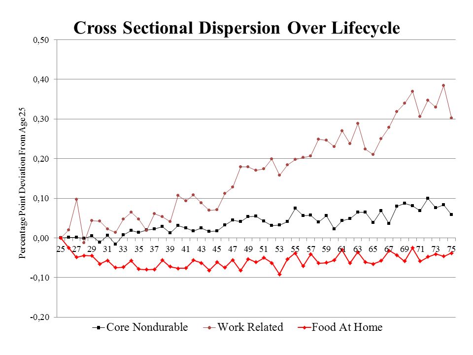
112. 112 What About Deaton-Paxson Fact? Examine lifecycle profile of cross sectional inequality by category Goods which have expenditures that increase with market work (due to home production or complementarity) should experience increasing dispersion when the dispersion of work increases. Portion of lifecycle profile of cross sectional inequality due to these goods does NOT inform researchers about: o Lifecycle profile of shocks to permanent income o Insurance mechanisms available to households

113. Dispersion of Propensity to Work Over Life Cycle

114. Cross Sectional Dispersion Over Lifecycle

116. Cross Sectional Dispersion Over Lifecycle: Figure 6b Core

117. Cross Sectional Dispersion Over Lifecycle: Figure 6b Core

118. Food, Transportation and Clothing Food is amenable to “Beckerian” home production (see Aguiar and Hurst 2005, 2007) No evidence of any decline in food intake over the lifecycle despite declining food expenditures. As opportunity cost of time declines later in life, households substitute towards home production of food (including more intense shopping for bargains). Data (and calibrated model) actual show food intake increases over the back half of the lifecycle

119. Work Related Expenses Transportation, Clothing and Food Away From Home are work related expenses: Lazear and Michael (1980) – Net out work related expenses (clothing and transportation) when making welfare calculations across people Banks et al (1998) and Battistin et al (2008) when measuring consumption changes of retirees Nelson (1989) and DeWeese and Norton (1991) comprising models of “clothing demand”

120. Level of Work Hours Over the Lifecycle

121. New Facts About Food, Clothing, and Transport Look at food away patterns at different types of establishments Look at changes in different amounts of transportation patterns using time use data Estimate “simple” demand systems and control directly for work status

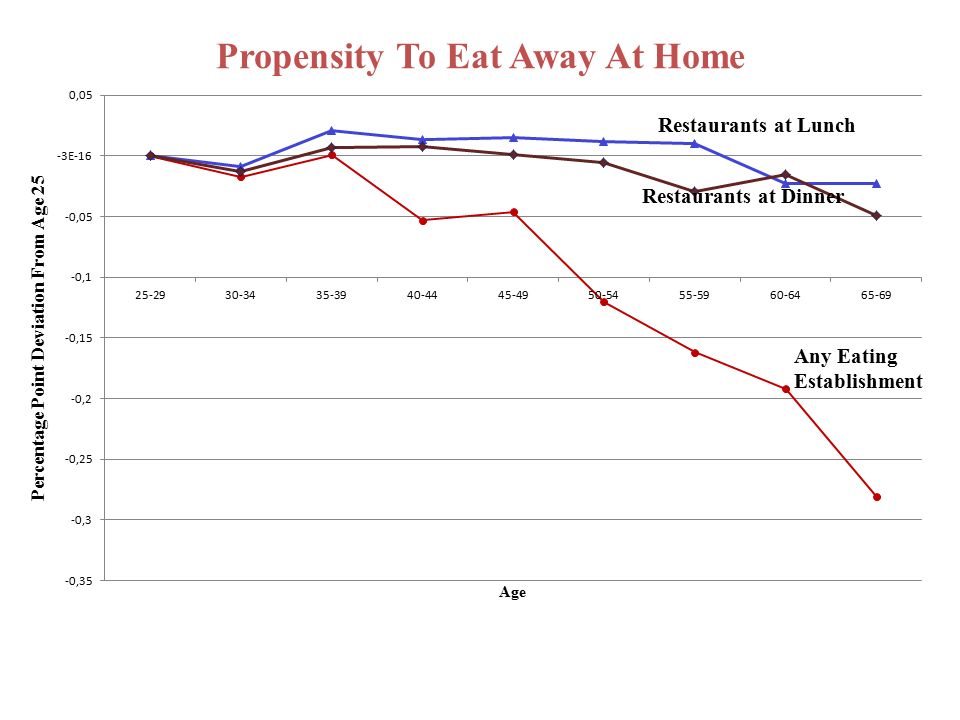
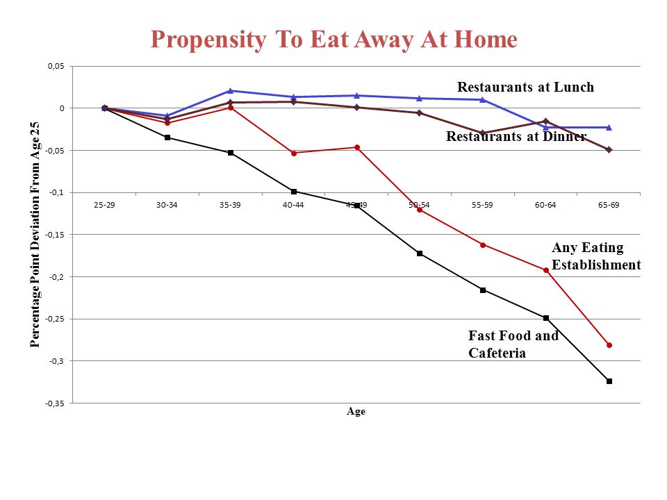
122. Propensity To Eat Away At Home

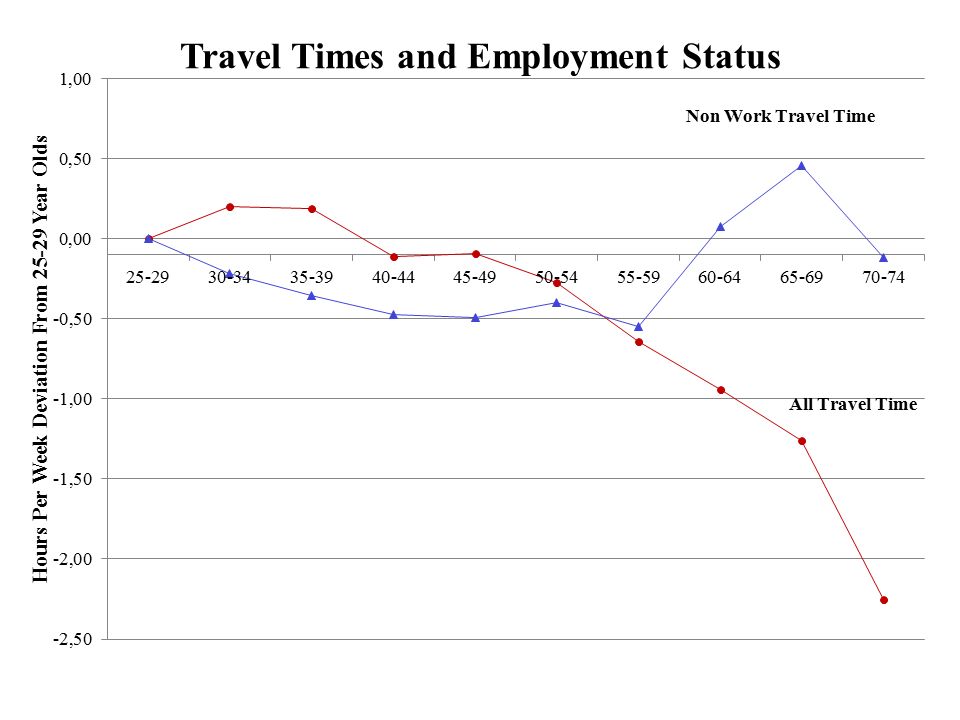
125. Travel Times and Employment Status

128. Control Directly For Work Status Estimate a demand system Control for labor supply (conditional on total expenditures) Estimate: 1)what consumption categories where spending is positively associated with market work 2)to what extent is the decline in spending on clothing, transportation and food away from home attributable to employment status.

129. Estimate Simple Demand System X it is total nondurable expenditures (less alcohol and tobacco, plus housing) for household i in year t. s it k is the share of expenditures in consumption category k out of X it P t k is the price index for consumption category k in year t L it is a vector of work status controls for household i in year t. Note:Instrument lnX it with household total income and education controls

130. 1. Simple Demand System Results Restrict sample to married households between age 25 and 50 Use two work status controls: Husband working? Wife working?

131. Simple Demand System Results Restrict sample to married households between age 25 and 50 Use two work status controls: Husband working? Wife working? Consumption CategoryHusband Work?Wife Work? Transportation(0.13) 0.014 (0.002) 0.014 (0.002) Clothing/P. Care (0.08) 0.003 (0.001)0.001 (0.001) Food Away From Home (0.06) 0.008 (0.001)0.005 (0.001)

132. Simple Demand System Results Restrict sample to married households between age 25 and 50 Use two work status controls: Husband working? Wife working? Consumption CategoryHusband Work?Wife Work? Transportation(0.13) 0.014 (0.002) 0.014 (0.002) Clothing/P. Care (0.08) 0.003 (0.001)0.001 (0.001) Food Away From Home (0.06) 0.008 (0.001)0.005 (0.001) Housing Services (0.34)-0.009 (0.003) -0.012 (0.002) Utilities (0.12)-0.005 (0.001) -0.003 (0.001) Food At Home(0.18)-0.016 (0.002) -0.013 (0.001) Entertainment(0.04) 0.000 (0.001)0.000 (0.001)

133. 2. Adding Work Controls To the Lifecycle Profile Married Sample, 25 – 75 Work Status Controls: 7 Dummies for Husband Weeks Worked 7 Dummies for Wife Weeks Worked 9 Dummies for Hours per week Husband Worked 9 Dummies for Hours per week Wife Worked Three Categories: Food (food at home and food away) Work Related Expenses (transportation and clothing) Core Non Durables (everything else) Ask: “How do work status controls effect lifecycle profiles?”

134. Demand Estimates, Transportation

135. Demand Estimates, Food Away

136. Demand Estimates, Clothing

137. Level of Lifecycle Expenditure

138. Level of Lifecycle Expenditure (Older Version)

139. What Does it Mean? Write down a model where households maximize utility with three consumption goods and leisure with the following constraints: one good (food) is amenable to home production one good (transport, clothes) are complements to market work there is a time budget constraint Assumptions: o conditional on work, income process is uncertain o take the lifecycle process of work as exogenous o assume that individual receives no utility for the lifecycle component of work related expenses. Other from the disaggregated consumption data (and home production functions), very similar procedure to Gourinchas and Parker.

140. Model: Household Income Risk While Working: Retirement/Disability Shock (R t ) Conditional on R t = 0, there is an age dependent hazard that next period R t+1 = 1.

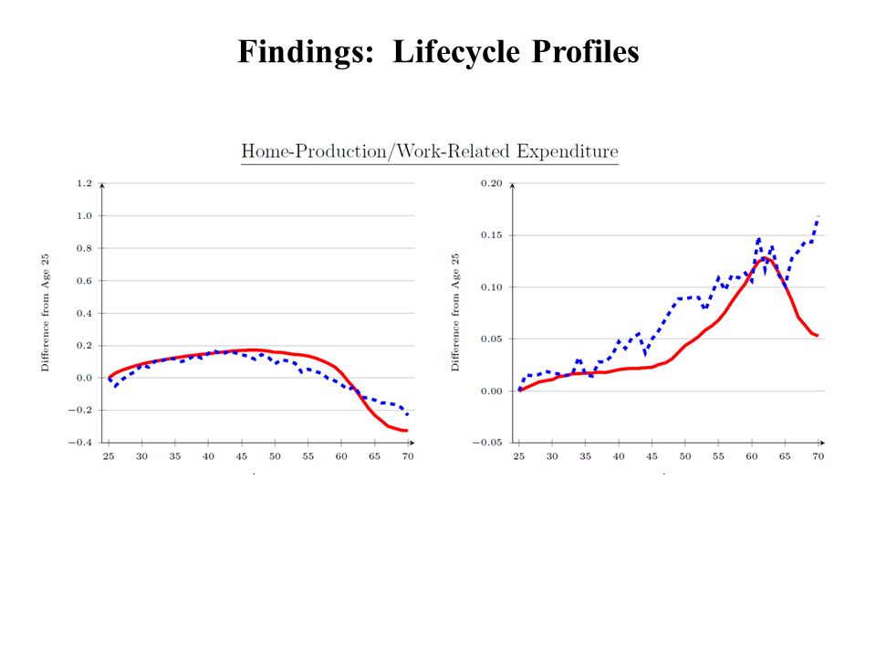
141. Model: Household Close the model with a standard representative competitive firm. Calibrate the model to match: average labor supply of prime age workers, lifecycle profile of spending on “core” and “home-production”/ “work-related” goods, the variance of spending on those goods and the coviariance.

142. Findings Households face much less risk than estimated by Gourinchas and Parker oCross sectional variation in core consumption is much less than cross sectional variance in total. oFind that permanent variance of income risk is 35% lower (0.047 vs. 0.073).

143. Findings: Lifecycle Profiles

146. Home Production vs. Non-Separable Preferences A Question: Does one need to model the home production sector formally? There is always a mapping between home production (non-separability between X and N through home production technology) and preferences (non-separability between X and N through preferences). oX = expenditures oN = labor However, to match the data, may need to have preference parameters change over time (or states). We will talk more about this in Topic 4.

147. Heckman (1974): Non-Separable Consumption and Leisure

148. Big Picture Wrap Up: Non Separabilities My belief: U(C,N) can be written as u(C) + v(N) However – we do not measure C directly: C = f(x,h) where h is directly related to N (through time budget constraint). We measure X and N in the data. X = f -1 (C,h(N)) Implication: U(X,N) cannot be written as U(X) + V(N).

149. A Short Summary Non Separabilities between X and N (expenditure and labor supply) are important. When is it important to implicitly model the home production sector? When changes to home production technology are important! When care about cross good predictions. When have actual consumption (intake) measures. For most applications, a reduced form assumption that X and N are non- separable can be important. Show a situation (with labor supply) where it may be useful to separate the home production sector separately from preferences.