1. Giuseppe Lancia University of Udine The phasing of heterozygous traits: Algorithms and Complexity

2. -The genomic age has allowed to look at ourselves in a detailed, comparative way -All humans are >99% identical at genome level -Small changes in a genome can make a big difference in how we look and who we are

3. What makes us different from each other? The answer is POLYMORPHISMS

4. This is true for humans as well as for other species

5. Polymorphisms are features existing in different “flavours”, that make us all look (and be) different Examples can be eye-color, blood type, hair, etc… In fact, polymorphisms in the way we look (phenotyes) are determined by polymorphisms in our genome

6. For a given polymorhism, say the eye-color, the possible forms are called alleles We all inherit two alleles (paternal and maternal) identical  HOMOZYGOUS If they are different  HETEROZYGOUS {

7. mother father child Homozygous

8. mother father child Homozygous mother father child Heterozygous Dominant Recessive

9. mother father child Homozygous mother father child Heterozygous mother father child Homozygous Dominant Recessive

10. mother father child Homozygous mother father child Heterozygous mother father child Homozygous Dominant Recessive

11. mother father child mother father child mother father child ?? ?? ?? ?? ?? ??

12. mother father child mother father child mother father child ?? ?? ?? ?? ?? ??

13. Single Single Nucleotide NucleotidePolymorphisms

14. At DNA level, a polymorphism is a sequence of nucleotides varying in a population. The shortest possible sequence has only 1 nucleotide, hence SNP S ingle N ucleotide P olymorphism (SNP)

15. At DNA level, a polymorphism is a sequence of nucleotides varying in a population. The shortest possible sequence has only 1 nucleotide, hence SNP S ingle N ucleotide P olymorphism (SNP) atcgg a ttagttagggcacaggacg g ac atcgg a ttagttagggcacaggacg t ac atcgg c ttagttagggcacaggacg t ac atcgg a ttagttagggcacaggacg g ac atcgg c ttagttagggcacaggacg t ac atcgg c ttagttagggcacaggacg g ac atcgg a ttagttagggcacaggacg t ac atcgg a ttagttagggcacaggacg g ac atcgg c ttagttagggcacaggacg g ac atcgg a ttagttagggcacaggacg g ac atcgg c ttagttagggcacaggacg g ac atcgg a ttagttagggcacaggacg g ac

16. - SNPs are predominant form of human variations atcgg a ttagttagggcacaggacg g ac atcgg a ttagttagggcacaggacg t ac atcgg c ttagttagggcacaggacg t ac atcgg a ttagttagggcacaggacg g ac atcgg c ttagttagggcacaggacg t ac atcgg c ttagttagggcacaggacg g ac atcgg a ttagttagggcacaggacg t ac atcgg a ttagttagggcacaggacg g ac atcgg c ttagttagggcacaggacg g ac atcgg a ttagttagggcacaggacg g ac atcgg c ttagttagggcacaggacg g ac atcgg a ttagttagggcacaggacg g ac - Used for drug design, study disease, forensic, evolutionary... - On average one every 1,000 bases

17. atcgg c ttagttagggcacaggacg t ac atcgg a ttagttagggcacaggacg g ac atcgg c ttagttagggcacaggacg t ac atcgg c ttagttagggcacaggacg g ac atcgg a ttagttagggcacaggacg t ac atcgg a ttagttagggcacaggacg t atcgg a ttagttagggcacaggacg g ac atcgg c ttagttagggcacaggacg g ac atcgg a ttagttagggcacaggacg g ac atcgg c ttagttagggcacaggacg g ac atcgg a ttagttagggcacaggacg g ac atcgg a ttagttagggcacaggacg t ac - SNPs are predominant form of human variations - Used for drug design, study disease, forensic, evolutionary... - On average one every 1,000 bases

18. ag at ct ag ct cg at ag cg ag cg ag - SNPs are predominant form of human variations - Used for drug design, study disease, forensic, evolutionary... - On average one every 1,000 bases

19. ag at ct ag ct cg at ag cg ag cg ag HAPLOTYPE HAPLOTYPE : chromosome content at SNP sites

20. ag at ct ag ct cg at ag cg ag cg ag HAPLOTYPE HAPLOTYPE : chromosome content at SNP sites GENOTYPE GENOTYPE : “union” of 2 haplotypes {c}{g,t} {a,c}{g,t} {a}{g} {a}{g,t} {a}{t} {a,c}{g}

21. ag at ct ag ct cg at ag cg ag cg ag {a,c}{g,t} {a}{g,t} {c}{g,t} {a}{g} {a}{t} {a,c}{g} CHANGE OF SYMBOLS CHANGE OF SYMBOLS : each SNP only two values in a population (bio). Call them 0 and 1. Also, call 2 the fact that a site is heterozygous HAPLOTYPE HAPLOTYPE: string over 0, 1 GENOTYPE GENOTYPE: string over 0, 1, 2

22. ag at ct ag ct cg at ag cg ag cg ag {a,c}{g,t} {a}{g,t} {c}{g,t} {a}{g} {a}{t} {a,c}{g} CHANGE OF SYMBOLS CHANGE OF SYMBOLS : each SNP only two values in a population (bio). Call them 0 and 1. Also, call 2 the fact that a site is heterozygous HAPLOTYPE HAPLOTYPE: string over 0, 1 GENOTYPE GENOTYPE: string over 0, 1, 2 where 0={0}, 1={1}, 2={0,1}

23. 10 11 01 10 01 00 11 10 00 10 00 10 02 22 10 12 11 20 CHANGE OF SYMBOLS CHANGE OF SYMBOLS : each SNP only two values in a population (bio). Call them 0 and 1. Also, call 2 the fact that a site is heterozygous HAPLOTYPE HAPLOTYPE: string over 0, 1 GENOTYPE GENOTYPE: string over 0, 1, 2 where 0={0}, 1={1}, 2={0,1}

24. 10 11 01 10 01 00 11 00 10 02 22 10 12 22 20 0 + 0 = --- 0 1 + 1 = --- 1 0 + 1 + 1 = 0 = --- --- 2 2 ALGEBRA OF HAPLOTYPES: Homozygous sites Heterozygous (ambiguous) sites

25. 12202 11101 10000 11100 10001 11001 10100 11000 10101 Phasing the alleles For k heterozygous (ambiguous) sites, there are 2 k-1 possible phasings

26. THE PHASING (or HAPLOTYPING) PROBLEM Given genotypes of k individuals, determine the phasings of all heterozygous sites. It is too expensive to determine haplotypes directly Much cheaper to determine genotypes, and then infer haplotypes in silico: This yields a set H, of (at most) 2k haplotypes. H is a resolution of G.

27. The input is GENOTYPE data 00011 11011 21221 22221 11221 INPUT: G = { 11221, 22221, 11011, 21221, 00011 }

28. The input is GENOTYPE data 11011 11101 00011 11101 11011 01101 11011 00011 11011 21221 22221 11221 OUTPUT: H = { 11011, 11101, 00011, 01101 } INPUT: G = { 11221, 22221, 11011, 21221, 00011 } Each genotype is resolved by two haplotypes We will define some objectives for H

29. - -without objectives/constraints, the haplotyping problem would be (mathematically)trivial OBJECTIVES 22021  00001 11011 E.g., always put 0 above and 1 below 12022  10000 11011 - -the objectives/constraints must be “driven by biology”

30. 2°) 2°) (parsimony): minimize |H| 1°) 1°) Clark’s inference rule 3°) Perfect Phylogeny 4°) Disease Association OBJECTIVES

31. Obj: Clark’s rule 1st

32. 1011001011 + ********** = 1221001212 known haplotype h known (ambiguos) genotype g Inference Rule for a compatible pair h, g

33. 1011001011 + 1101001110 = 1221001212 known haplotype h known (ambiguos) genotype g Inference Rule for a compatible pair h, g new (derived) haplotype h’ We write h + h’ = g

34. 1st Objective (Clark, 1990) 1. Start with H = “bootstrap” haplotypes 2. while Clark’s rule applies to a pair (h, g) in H x G 3. apply the rule to any such (h, g) obtaining h’ 4. set H = H + {h’} and G = G - {g} 5. end while

35. If, at end, G is empty, SUCCESS, otherwise FAILURE Step 3 is non-deterministic 1st Objective (Clark, 1990) 1. Start with H = “bootstrap” haplotypes 2. while Clark’s rule applies to a pair (h, g) in H x G 3. apply the rule to any such (h, g) obtaining h’ 4. set H = H + {h’} and G = G - {g} 5. end while

36. If, at end, G is empty, SUCCESS, otherwise FAILURE Step 3 is non-deterministic 1st Objective (Clark, 1990) 1. Start with H = “bootstrap” haplotypes 2. while Clark’s rule applies to a pair (h, g) in H x G 3. apply the rule to any such (h, g) obtaining h’ 4. set H = H + {h’} and G = G - {g} 5. end while 0000 1000 2200 1122

37. If, at end, G is empty, SUCCESS, otherwise FAILURE Step 3 is non-deterministic 1st Objective (Clark, 1990) 1. Start with H = “bootstrap” haplotypes 2. while Clark’s rule applies to a pair (h, g) in H x G 3. apply the rule to any such (h, g) obtaining h’ 4. set H = H + {h’} and G = G - {g} 5. end while 0000 1000 2200 1122 1100

38. If, at end, G is empty, SUCCESS, otherwise FAILURE Step 3 is non-deterministic 0000 1000 2200 1122 1100 1111 SUCCESS 1st Objective (Clark, 1990) 1. Start with H = “bootstrap” haplotypes 2. while Clark’s rule applies to a pair (h, g) in H x G 3. apply the rule to any such (h, g) obtaining h’ 4. set H = H + {h’} and G = G - {g} 5. end while

39. If, at end, G is empty, SUCCESS, otherwise FAILURE Step 3 is non-deterministic 1st Objective (Clark, 1990) 1. Start with H = “bootstrap” haplotypes 2. while Clark’s rule applies to a pair (h, g) in H x G 3. apply the rule to any such (h, g) obtaining h’ 4. set H = H + {h’} and G = G - {g} 5. end while 0000 1000 2200 1122

40. If, at end, G is empty, SUCCESS, otherwise FAILURE Step 3 is non-deterministic 1st Objective (Clark, 1990) 1. Start with H = “bootstrap” haplotypes 2. while Clark’s rule applies to a pair (h, g) in H x G 3. apply the rule to any such (h, g) obtaining h’ 4. set H = H + {h’} and G = G - {g} 5. end while 0000 1000 2200 1122 0100

41. If, at end, G is empty, SUCCESS, otherwise FAILURE Step 3 is non-deterministic 0000 1000 2200 1122 0100 FAILURE (can’t resolve 1122 ) 1st Objective (Clark, 1990) 1. Start with H = “bootstrap” haplotypes 2. while Clark’s rule applies to a pair (h, g) in H x G 3. apply the rule to any such (h, g) obtaining h’ 4. set H = H + {h’} and G = G - {g} 5. end while

42. 1. Start with H = “bootstrap” haplotypes 2. while Clark’s rule applies to a pair (h, g) in H x G 3. apply the rule to any such (h, g) obtaining h’ 4. set H = H + {h’} and G = G - {g} 5. end while If, at end, G is empty, SUCCESS, otherwise FAILURE Step 3 is non-deterministic: the algorithm could end without explaining all genotypes even if an explanation was possible. The number of genotypes solved depends on order of application. 1st Objective (Clark, 1990) OBJ: find order of application rule that leaves the fewest elements in G

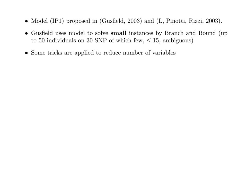
43. The problem was studied by Gusfield (ISMB 2000, and Journal of Comp. Biol., 2001) - problem is APX-hard - it corresponds to finding largest forest in a graph with haplotypes as nodes and arcs for possible derivations -solved via ILP of exponential-size (practical for small real instances)

44. Obj: Max Parsimony 2nd

45. - Clark conjectured solution (when found) uses min # of haplotypes - this is clearly false - solution with few haplotypes is biologically relevant (as we all descend from a small set of ancestors)

46. 011 101 111 011 000 010 001 010 011 111

47. 011 101 111 011 000 010 001 010 011 111 022 222 012 221 011 111 022 211 012 022 012 222

48. minimize |H| 2nd Objective (parsimony) 2nd Objective (parsimony) :

49. 1. The problem is APX-Hard Reduction from VERTEX-COVER

50. A B C D E

51. A B C D E A B C D E *

52. A B C D E AB BC AE DE AD

53. A B C D E A B C D E * AB BC AE DE AD A B C D E

54. A B C D E A B C D E * AB 2 2 BC 2 2 AE 2 2 DE 2 2 AD 2 2 A B C D E

55. A B C D E A B C D E * AB 2 2 BC 2 2 AE 2 2 DE 2 2 AD 2 2 A 0 B 0 C 0 D 0 E 0

56. A B C D E A B C D E * AB 2 2 2 BC 2 2 2 AE 2 2 2 DE 2 2 2 AD 2 2 2 A 0 0 B 0 0 C 0 0 D 0 0 E 0 0

57. A B C D E A B C D E * AB 2 2 1 1 1 2 BC 1 2 2 1 1 2 AE 2 1 1 1 2 2 DE 1 1 1 2 2 2 AD 2 1 1 2 1 2 A 0 1 1 1 1 0 B 1 0 1 1 1 0 C 1 1 0 1 1 0 D 1 1 1 0 1 0 E 1 1 1 1 0 0

58. A B C D E A B C D E * AB 2 2 1 1 1 2 BC 1 2 2 1 1 2 AE 2 1 1 1 2 2 DE 1 1 1 2 2 2 AD 2 1 1 2 1 2 A 0 1 1 1 1 0 B 1 0 1 1 1 0 C 1 1 0 1 1 0 D 1 1 1 0 1 0 E 1 1 1 1 0 0 G = (V,E) has a node cover X of size k  there is a set H of |V | + k haplotypes that explain all genotypes

59. A B C D E A B C D E * AB 2 2 1 1 1 2 BC 1 2 2 1 1 2 AE 2 1 1 1 2 2 DE 1 1 1 2 2 2 AD 2 1 1 2 1 2 A 0 1 1 1 1 0 B 1 0 1 1 1 0 C 1 1 0 1 1 0 D 1 1 1 0 1 0 E 1 1 1 1 0 0 G = (V,E) has a node cover X of size k  there is a set H of |V | + k haplotypes that explain all genotypes

60. A B C D E A B C D E * AB 2 2 1 1 1 2 BC 1 2 2 1 1 2 AE 2 1 1 1 2 2 DE 1 1 1 2 2 2 AD 2 1 1 2 1 2 A 0 1 1 1 1 0 B 1 0 1 1 1 0 C 1 1 0 1 1 0 D 1 1 1 0 1 0 E 1 1 1 1 0 0 A’ 0 1 1 1 1 1 B’ 1 0 1 1 1 1 E’ 1 1 1 1 0 1 G = (V,E) has a node cover X of size k  there is a set H of |V | + k haplotypes that explain all genotypes

61. A basic ILP formulation

62. Expand your input G in all possible ways 220 120 022 A basic ILP formulation

63. Expand your input G in all possible ways 010 + 100, 000 + 110 100 + 110 000 + 011, 001 + 010 220 120 022 A basic ILP formulation

64. Expand your input G in all possible ways 010 + 100, 000 + 110 100 + 110 000 + 011, 001 + 010 220 120 022 A basic ILP formulation

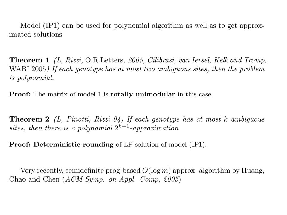
65. The resulting Integer Program (IP1):

67. Other ILP formulation are possible. E.g. POLY-SIZE ILP formulations

69. Obj: Perfect Phylogeny 3rd

70. - Parsimony does not take into account mutations/evolution of haplotypes - parsimony is very relialable on “small” haplotype blocks - when haplotypes are large (span several SNPs, we should consider evolutionionary events and recombination) - the cleanest model for evolution is the perfect phylogeny

71. - A phylogeny expalains set of binary features (e.g. flies, has fur…) with a tree - Leaf nodes are labeled with species - Each feature labels an edge leading to a subtree that possesses it perfect phylogeny 3rd objective is based on perfect phylogeny

72. - A phylogeny expalains set of binary features (e.g. flies, has fur…) with a tree - Leaf nodes are labeled with species - Each feature labels an edge leading to a subtree that possesses it has 2 legs perfect phylogeny 3rd objective is based on perfect phylogeny has tail flies

73. - A phylogeny expalains set of binary features (e.g. flies, has fur…) with a tree - Leaf nodes are labeled with species - Each feature labels an edge leading to a subtree that possesses it has 2 legs But…a new species may come along so that no Perfect phylogeny is possible… has tail flies

74. Theorem Theorem: such matrix has p.p. iff there is not a 00 4x2 minor 10 01 11 Human 1 0 0 Mouse 0 1 0 Spider 0 0 0 Eagle 1 0 1 two legs tail flies

75. Theorem Theorem: such matrix has p.p. iff there is not a 00 4x2 minor 10 01 11 Human 1 0 0 Mouse 0 1 0 Spider 0 0 0 Eagle 1 0 1 Mickey mouse 1 1 0 two legs tail flies

76. We can consider each SNP as a binary feature Objective: Objective: We want the solution to admit a perfect phylogeny (Rationale : we assume haplotypes have evolved independently along a tree)

77. We can consider each SNP as a binary feature Objective: Objective: We want the solution to admit a perfect phylogeny (Rationale : we assume haplotypes have evolved independently along a tree) 0 1 2 0 2 1 0 2 2 0

78. We can consider each SNP as a binary feature Objective: Objective: We want the solution to admit a perfect phylogeny (Rationale : we assume haplotypes have evolved independently along a tree) 0 1 0 0 0 1 1 0 1 1 0 1 0 1 0 0 1 0 0 0 0 0 1 0 0 1 2 0 2 1 0 2 2 0

79. We can consider each SNP as a binary feature Objective: Objective: We want the solution to admit a perfect phylogeny (Rationale : we assume haplotypes have evolved independently along a tree) 0 1 2 0 2 1 0 2 2 0 0 1 0 0 0 1 1 0 1 1 0 1 0 1 0 0 1 0 0 0 0 0 1 0 NOT a perfect phylogeny solution !

80. We can consider each SNP as a binary feature Objective: Objective: We want the solution to admit a perfect phylogeny (Rationale : we assume haplotypes have evolved independently along a tree) 0 1 2 0 0 1 0 2 0 0 0 2

81. We can consider each SNP as a binary feature Objective: Objective: We want the solution to admit a perfect phylogeny (Rationale : we assume haplotypes have evolved independently along a tree) 0 1 2 0 0 1 0 2 0 0 0 2 0 1 0 0 0 1 1 0 0 1 0 0 1 1 0 1 0 0 0 0 0 1 A perfect phylogeny

82. Theorem: The Perfect Phylogeny Haplotyping problem is polynomial

83. Algorithms are of combinatorial nature - There is a graph for which SNPs are columns and edges are of two types (forced and free) - forced edges connect pairs of SNPs that must be phased in the same way 22  00 + 11 or 22  01 + 10 - a complex visit of the graph decides how to phase free SNPs

84. Obj: Disease Association 4th

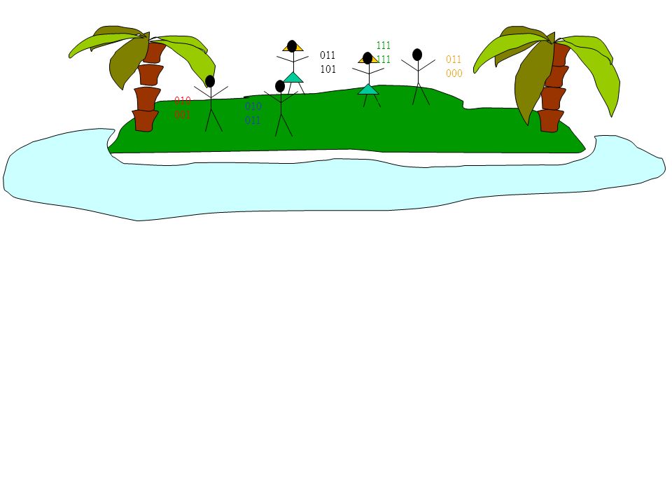
85. Some diseases may be due to a gene which has “faulty” configurations RECESSIVE DISEASE (e.g. cystic fibrosis, sickle cell anemia): to be diseased one must have both copies faulty. With one copy one is a carrier of the disease DOMINANT DISEASE (e.g. Huntington’s disease, Marfan’s syndrome): to be diseased it is enough to have one faulty copy Two individuals of which one is healthy and the other diseased may have the same genotype. The explanation of the disease lies in a difference in their haplotypes

86. 00011 02011 21221 02201 11221 INPUT: GD = { 11221,21221,02011 }, GH = {11221,02201,00011} 11221

87. 11011 11101 00011 01101 00001 11011 01101 01011 00011 02011 21221 02201 11221 OUTPUT: H = { 11011,01011,00001,11111,11101,00011,01101 } H contains H D, s.t. each diseased has >=1 haplotype in H D and each healty none INPUT: GD = { 11221,21221,02011 }, GH = {11221,02201,00011} 11001 11111 11221

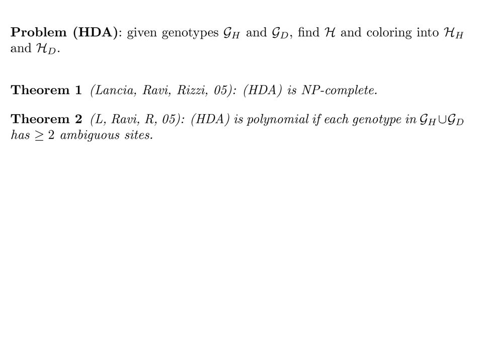
89. Theorem 1 is proved via a reduction from 3 SAT Theorem 2 has a mathematical proof (coloring argument) with little relation to biology: There is R (depending on input) s.t. a haplotype is healthy if the sum of its bits is congruent to R modulo 3 This means the model must be refined!

91. Summary: - haplotyping in-silico needed for economical reasons - several objectives, all biologically driven - nice combinatorial problems (mostly from binary nature of SNPs) - these problems are technology-dependant and may become obsolete (hopefully after we have retired)

92. Thanks