1. Fast Fourier Transform 向 华 武汉大学数学与统计学院

2. Fast Fourier Transform The Fast Fourier Transform (FFT) is a very efficient algorithm for performing a discrete Fourier transform A.C.Clairaut,cosine-only finite Fourier series(1754),J.L.Lagrange,sine-only series(1762),Bernoulli,a series of sine and cosine.FFT principle first used by Gauss in 1805? FFT algorithm published by Cooley & Tukey in 1965 In 1969, the 2048 point analysis of a seismic trace took 13 ½ hours. Using the FFT, the same task on the same machine took 2.4 seconds!

3. Fourier 变换 : 存在的条件 : 反变换 : Jean Baptiste Joseph Fourier (1768 - 1830) 注意不同文献中的定义，特别是系数,exp(-i2πkx) …

4. 当 g(x) 为实函数

5. delta 函数 t (t)(t)   TopHat 函数

6.       cos(  0 t) t  cosine 函数 sine 函数

7. 位移性质 : 相似性质 : a-a

8. energy theorem, Rayleigh’s theorem The zero frequency point 反变换 : 代入

9. 常用的 Fourier 变换

10. 连续傅立叶变换 (Continuous Fourier Transform) 离散傅立叶变换 (Discrete Fourier Transform) where For u=0,1,2,…,N-1 For x=0,1,2,…,N-1 连续傅立叶变换 (Continuous Fourier Transform) 离散傅立叶变换 (Discrete Fourier Transform) 常用的其他定义

11. 连续 Fourier 变换 (Continuous Fourier Transform) 反变换 DFT: IDFT:

12. 矩阵形式的 DFT

13. omega = exp(-2*pi*i/n); j = 0:n-1; k = j'; F = omega.^(k*j); % an easier,and quicker, way to generate F is F = fft(eye(n));

14. Requires N 2 complex multiplies and N(N-1) complex additions 离散 Fourier 变换 (DFT) ( 此处定义与教材和 MATLAB 保持一致 ) 对称性 : 周期性 : W N =e -i 2π/N

15. 两个长度为 N/2 的 DFT 之和

16. Cross feed of G[k] and H[k] in flow diagram is called a “ butterfly ”, due to the shape or simplify: X[0…7] x[0,2,4,6] x[1,3,5,7] N/2 DFT N/2 DFT

18. 对 N=8 ， DecimalBinary Decimal 0000 0 1001 1004 2010 2 3011 1106 4100 0011 5101 5 6110 0113 7111 7 bit reversal (0, 1, 2, 3, 4, 5, 6, 7 is reordered to 0, 4, 2, 6, 1, 5, 3, 7)

19. 因为 W N/2 = -1, Ｘ k 0 和 Ｘ k 1 具有周期 N/2, There are N/2 butterflies for this stage of the FFT, and each butterfly requires one multiplication Diagrammatically (butterfly), The splitting of {X k } into two half-size DFTs can be repeated on Ｘ k 0 and Ｘ k 1 themselves,

20. The FFT for eight data values d 1,d 2, …,d 7 proceeds as follows. 参考 P55, C.W.Ueberhuber,Numerical Computation 2,Springer 1995.

21. –{ Ｘ k 00 } is the N/4-point DFT of {x 0, x 4, …, x N-4 }, –{ Ｘ k 01 } is the N/4-point DFT of {x 2, x 6, …, x N-2 }, –{ Ｘ k 10 } is the N/4-point DFT of {x 1, x 5, …, x N-3 }, –{ Ｘ k 11 } is the N/4-point DFT of {x 3, x 7, …, x N-1 }.

22. 定义 c=[0 2 4 6 1 3 5 7] 这里四页内容选自 G.H.Golub,C.F.Van Loan 的《矩阵计算》。

25. function y=fft(x,n) if n=1 y=x else m=n/2; w=e -i2πn y T =fft(x(0:2:n),m) y B =fft(x(1:2:n),m) d=[1,w,…,w m-1 ] T z=d.*y B y=[y T +z; y B +z] end 设 n=2 t 它有一种非循环的实现方式，可用 的分解来描述： 其中 称为反位置换 (bit reversal permutation).

26. fftgui(y) 产生 4 个 plots: real(y), imag(y), real(fft(y)), imag(fft(y)) print -deps FftGui.eps print – depsc2 FftGui.eps 以下部分内容选自 Moler 的书《 Numerical Computing with Matlab 》。

27. y 0 =1,y 1 =…=y n-1 =0,

28. y 0 =0,y 1 =1,y 2 =…=y n-1 =0,

29. FFT is the sum of two sinusoids

30. The Nyquist point

31. Some symmetries in the FFT. Ignoring the first point in each plot, the real part is symmetric about the Nyquist point and the imaginary part is antisymmetric about the Nyquist point. More precisely, 若 y 是长度为 n 的实向量,Y=fft(y), 则 real(Y 0 ) = ∑y j imag(Y 0 ) = 0 real(Y j ) = real(Y n-j ), j=1,…,n/2 imag(Y j ) = -imag(Y n-j ),j=1,…,n/2

32. 697 770 852 941 1209 1336 1477 % the sampling rate. Fs = 32768; t = 0:1/Fs:0.25; % the button in position (k,j) for k=1:4 for j=1:3 y1 = sin(2*pi*fr(k)*t); y2 = sin(2*pi*fc(j)*t); y = (y1 + y2)/2; input('Press any key:)'); sound(y,Fs) end

34. load sunspot.dat t = sunspot(:,1)'; wolfer = sunspot(:,2)'; n = length(wolfer); c = polyfit(t,wolfer,1); trend = polyval(c,t); plot(t,[wolfer; trend],'-', t,wolfer,'k.') For centuries, people have noted that the face of the sun is not constant or uniform in appearance, but that darker regions appear at random locations on a cyclical basis. In1848,Rudolf Wolfer proposed a rule that combined the number and size of these sunspots into a single index.

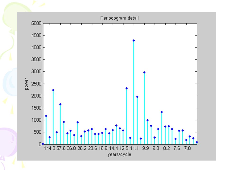
36. y = wolfer - trend; Y = fft(y); Fs = 1; % Sample rate f = (0:n/2)*Fs/n; pow = abs(Y(1:n/2+1)); plot([f; f],[0*pow; pow],'c-', … f,pow,'b.',... 'linewidth',2, 'markersize',16) Now subtract off the linear trend and take the FFT.

39. plot(fft(eye(17))) axis square

40. Chebyshev Polynomial 扩充到复平面 扩充到 |z|>1 递推关系 : 满足微分方程 : 第二类 Chebyshev 多项式

41. shg,hold on fplot('x',[-1,1]) fplot('2*x^2-1',[-1,1]) fplot('4*x^3-3*x',[-1,1]) fplot('8*x^4-8*x^2+1',[-1,1]) fplot('16*x^5-20*x^3+5*x',[-1,1])

42. “We do not make things, We make things better.”