1. Sensors Ioannis Stamos

2. Perspective projection

3. Ioannis Stamos – CSCI 493.69 F08 Pinhole & the Perspective Projection SCREEN SCENE (x,y) Is there an image being formed on the screen?

4. Ioannis Stamos – CSCI 493.69 F08 Pinhole Object Pinhole camera Pinhole Camera “Camera obscura” – known since antiquity Image Image plane

5. Ioannis Stamos – CSCI 493.69 F08 Perspective Camera (X,Y,Z) (x,y,z) Center of Projection r r’ r =[x,y,z] T r’=[X,Y,Z] T r/f=r’/Z f: effective focal length: distance of image plane from O. x=f * X/Z y=f * Y/Z z=f From Trucco & Verri

6. Ioannis Stamos – CSCI 493.69 F08 Magnification (X,Y,Z) (x,y) Center of Projection (X+dX,Y+dY,Z) (x+dx,y+dy) x/f=X/Z y/f=Y/Z (x+dx)/f=(X+dX)/Z (y+dy)/z=(Y+dY)/Z dx/f=dX/Z dy/f=dY/Z => d d’ From Trucco & Verri

7. Ioannis Stamos – CSCI 493.69 F08 Magnification (X,Y,Z) (x,y) Center of Projection (X+dX,Y+dY,Z) (x+dx,y+dy) d d’ Magnification: |m|=||d’||/||d||=|f/Z| or m=f/Z m is negative when image is inverted… From Trucco & Verri

8. Ioannis Stamos – CSCI 493.69 F08 Implications For Perception* * A Cartoon Epistemology: http://cns-alumni.bu.edu/~slehar/cartoonepist/cartoonepist.html Same size things get smaller, we hardly notice… Parallel lines meet at a point…

9. Ioannis Stamos – CSCI 493.69 F08 Vanishing Points (from NALWA)

10. Ioannis Stamos – CSCI 493.69 F08 Vanishing points VPL VPR H VP 1 VP 2 VP 3 Different directions correspond to different vanishing points Marc Pollefeys

11. 3D is different…

12. 3D Data Types: Volumetric Data Regularly-spaced grid in (x,y,z): “voxels” For each grid cell, store Occupancy (binary: occupied / empty) Density Other properties Popular in medical imaging CAT scans MRI

13. 3D Data Types: Surface Data Polyhedral Piecewise planar Polygons connected together Most popular: “triangle meshes” Smooth Higher-order (quadratic, cubic, etc.) curves Bézier patches, splines, NURBS, subdivision surfaces, etc.

14. 2½-D Data Image: stores an intensity / color along each of a set of regularly-spaced rays in space Range image: stores a depth along each of a set of regularly-spaced rays in space Not a complete 3D description: does not store objects occluded (from some viewpoint) View-dependent scene description

15. 2½-D Data This is what most sensors / algorithms really return Advantages Uniform parameterization Adjacency / connectivity information Disadvantages Does not represent entire object View dependent

16. 2½-D Data Range images Range surfaces Depth images Depth maps Height fields 2½-D images Surface profiles xyz maps …

17. Range Acquisition Taxonomy Range acquisition Contact Transmissive Reflective Non-optical Optical Industrial CT Mechanical (CMM, jointed arm) Radar Sonar Ultrasound MRI Ultrasonic trackers Magnetic trackers Inertial (gyroscope, accelerometer)

18. Range Acquisition Taxonomy Optical methods Passive Active Shape from X: stereomotionshadingtexturefocusdefocus Active variants of passive methods Stereo w. projected texture Active depth from defocus Photometric stereo Time of flight Triangulation

19. Optical Range Acquisition Methods Advantages: Non-contact Safe Usually inexpensive Usually fast Disadvantages: Sensitive to transparency Confused by specularity and interreflection Texture (helps some methods, hurts others)

20. Stereo Find feature in one image, search along epipolar line in other image for correspondence

21. Stereo Vision depth map

22. Triangulation f T Z P plpl prpr OlOl OrOr Left CameraRight Camera X-axis Z-axis clcl crcr Fixation Point:Infinity. Parallel optical axes. Calibrated Cameras Similar triangles: d:disparity (difference in retinal positions). T:baseline. Depth (Z) is inversely proportional to d (fixation at infinity)

23. Traditional Stereo  Inherent problems of stereo:  Need textured surfaces  Matching problem  Baseline trade-off  Unstructured point set  However  Cheap (price, weight, size)  Mobile  Depth plus Color Sparse estimates Unreliable results

24. Why More Than 2 Views? Baseline Too short – low accuracy Too long – matching becomes hard

25. Multibaseline Stereo [ Okutami & Kanade]

26. Shape from Motion “Limiting case” of multibaseline stereo Track a feature in a video sequence For n frames and f features, have 2  n  f knowns, 6  n+3  f unknowns

27. Photometric Stereo Setup [Rushmeier et al., 1997]

28. Photometric Stereo Use multiple light sources to resolve ambiguity In surface orientation. Note: Scene does not move – Correspondence between points in different images is easy! Notation: Direction of source i: or Image intensity produced by source i:

29. Lambertian Surfaces (special case) orientation albedo Use THREE sources in directions Image Intensities measured at point (x,y):

30. Photometric Stereo: RESULT orientation albedo INPUT

31. Data Acquisition Example Color Image of Thomas Hunter Building, New York City. Range Image of same building. One million 3D points. Pseudocolor corresponds to laser intensity.

32. Time-of-flight scanners

33. DataAcquisition Spot laser scanner. Time of flight. Max Range: 100 meters. Scanning time: 16 minutes for one million points. Accuracy: ~6mm per range point

34. DataAcquisition Leica ScanStation 2 Spherical field of view. Registered color camera. Max Range: 300 meters. Scanning time: 2-3 times faster Accuracy: ~5mm per range point

35. Data Acquisition, Leica Scan Station 2, Park Avenue and 70 th Street, NY

36. Cyclone view and Cyrax Video

37. Pulsed Time of Flight Send out pulse of light (usually laser), time how long it takes to return

38. Pulsed Time of Flight Advantages: Large working volume (more than 100 m.) Disadvantages: Not-so-great accuracy (at best ~5 mm.) Requires getting timing to ~30 picoseconds Does not scale with working volume Often used for scanning buildings, rooms, archeological sites, etc.

39. Optical Triangulation Lens Sheet of light CCD array Sources of error: 1) grazing angle, 2) object boundaries.

40. Optical Triangulation Lens Sheet of light CCD array Sources of error: 1) grazing angle, 2) object boundaries.

41. Active Optical Triangulation Xc Yc Zc Image Light Stripe System. Light Plane: AX+BY+CZ+D=0 (in camera frame) Image Point: x=f X/Z, y=f Y/Z (perspective) Triangulation: Z=-D f/(A x + B y + C f) Move light stripe or object.

42. Triangulation

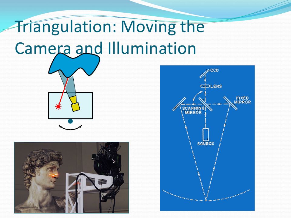
43. Triangulation: Moving the Camera and Illumination Moving independently leads to problems with focus, resolution Most scanners mount camera and light source rigidly, move them as a unit

44. Triangulation: Moving the Camera and Illumination

46. The Digital Michelangelo Project

47. Marc Levoy (Stanford) calibrated motions pitch (yellow) pan (blue) horizontal translation (orange) uncalibrated motions vertical translation remounting the scan head moving the entire gantry

48. Scanner design 4 motorized axes laser, range camera, white light, and color camera truss extensions for tall statues

49. Scanning the David height of gantry: 7.5 meters weight of gantry: 800 kilograms

50. Triangulation Scanner Issues Accuracy proportional to working volume (typical is ~1000:1) Scales down to small working volume (e.g. 5 cm. working volume, 50  m. accuracy) Does not scale up (baseline too large…) Two-line-of-sight problem (shadowing from either camera or laser) Triangulation angle: non-uniform resolution if too small, shadowing if too big (useful range: 15  -30  )

51. Triangulation Scanner Issues Accuracy proportional to working volume (typical is ~1000:1) Scales down to small working volume (e.g. 5 cm. working volume, 50  m. accuracy) Does not scale up (baseline too large…) Two-line-of-sight problem (shadowing from either camera or laser) Triangulation angle: non-uniform resolution if too small, shadowing if too big (useful range: 15  -30  )

52. Multi-Stripe Triangulation To go faster, project multiple stripes But which stripe is which? Answer #1: assume surface continuity

53. Multi-Stripe Triangulation To go faster, project multiple stripes But which stripe is which? Answer #2: colored stripes (or dots)

54. Multi-Stripe Triangulation To go faster, project multiple stripes But which stripe is which? Answer #3: time-coded stripes

55. Time-Coded Light Patterns Assign each stripe a unique illumination code over time [Posdamer 82] Space Time

56. Laser-based Sensing  Provides solutions  Dense & reliable  Regular grid  But  Complex & large point sets  Redundant point sets  No color information (explain this)  Expensive, non-mobile Adjacency info Mesh

57. Major Issues  Registration of point sets  Global and coherent geometry  remove redundancy  handle holes  handle all types of geometries  Handle complexity  Fast Rendering

58. Representations of 3D Scenes Geometry and Material Geometry and Images Images with Depth Colored Voxels Light-Field/Lumigraph Panorama with Depth Complete description Traditional texture mapping Scene as a light source Global Geometry Local Geometry False Geometry Panorama No/Approx. Geometry Facade

59. Head of Michelangelo’s David photograph1.0 mm computer model

60. David’s left eye holes from Michelangelo’s drillartifacts from space carving noise from laser scatter 0.25 mm modelphotograph

61. IBM’s Pietà Project Michelangelo’s “Florentine Pietà” Late work (1550s) Partially destroyed by Michelangelo, recreated by his student Currently in the Museo dell’Opera del Duomo in Florence

62. Scanner Visual Interface “Virtuoso” Active multibaseline stereo Projector (stripe pattern), 6 B&W cameras, 1 color camera Augmented with 5 extra “point” light sources for photometric stereo (active shape from shading)

63. Data Range data has 2 mm spacing, 0.1mm noise Each range image: 10,000 points, 20  20 cm Color data: 5 images with controlled lighting, 1280  960, 0.5 mm resolution Total of 770 scans, 7.2 million points

64. Scanning Final scan June 1998, completed July 1999 Total scanning time: 90 hours over 14 days (includes equipment setup time)

65. Results

66. HUNTER COLLEGE (our work): Segmented Planar Area. Exterior and Interior borders shown. Interior border. Range sensing direction. Each Segmented Planar Area is shown with different color for clarity. Exterior border. Intersection line.

67. HUNTER COLLEGE

68. HUNTER COLLEGE: Final result – 24 scan pairs ~600 lines per scan

69. HUNTER COLLEGE: Matching 3D with 2D imagery 3D parallelepipeds 2D rectangles Matches shown in blue

70. HUNTER COLLEGE: Virtual (synthetic) scene views

71. Virtual (synthetic) scene views