1. Image Restoration The main aim of restoration is to improve an image in some predefined way. Image Enhancement is a subjective process whereas Image restoration tries to reconstruct or recover an image which was degraded using a priori knowledge of degradation. Here we model the degradation and apply the inverse process to recover the original image. Enhancement techniques take advantage of the psychophysical aspects of human visual system. (eg) contrast stretching is an enhancement method as it is concerned with the pleasing aspects of a viewer, whereas removal of image blur is a restoration process.

2. Model of Image Degradation / Restoration Process In this model, we assume that there is an additive noise term, operating on an input image f(x,y) to produce a degraded image g(x,y). Given g(x,y) and some information about degradation function H, and knowledge about noise term η(x,y). The aim of restoration is to get an estimate f(x,y) of original image. The more we know about H and term η, we get better results.

3. Model of Image Degradation / Restoration Process Here H is a linear, position-invariant process. The degraded image is given as: g(x,y) = h(x,y)*f(x,y) + η(x,y) Here h(x,y) is the spatial representation of the degradation function. The symbol * indicates convolution. The convolution in spatial domain is equal to multiplication in frequency domain. In Frequency domain we have: G(u,v) = H(u,v)F(u,v) + N(u,v) Here capital letters are the Fourier transforms of the corresponding terms. For simplicity, we consider the case of H being the identity operator.

5. Origin of Noise Noise in a digital image arises mainly due to acquisition (digitization) and / or transmission. Environmental conditions, quality of sensing elements, interference in the transmission channel, lightning and atmospheric disturbance are some examples.

6. Properties of Noise When the Fourier spectrum of noise is constant, the noise is called a white noise. This is similar to white light, which contains nearly all frequencies in the visible spectrum in equal quantities. Fourier spectrum of a function containing all frequencies in equal proportions is a constant. We assume that noise is independent of coordinates, and it is uncorrelated with respect to the pixel values.

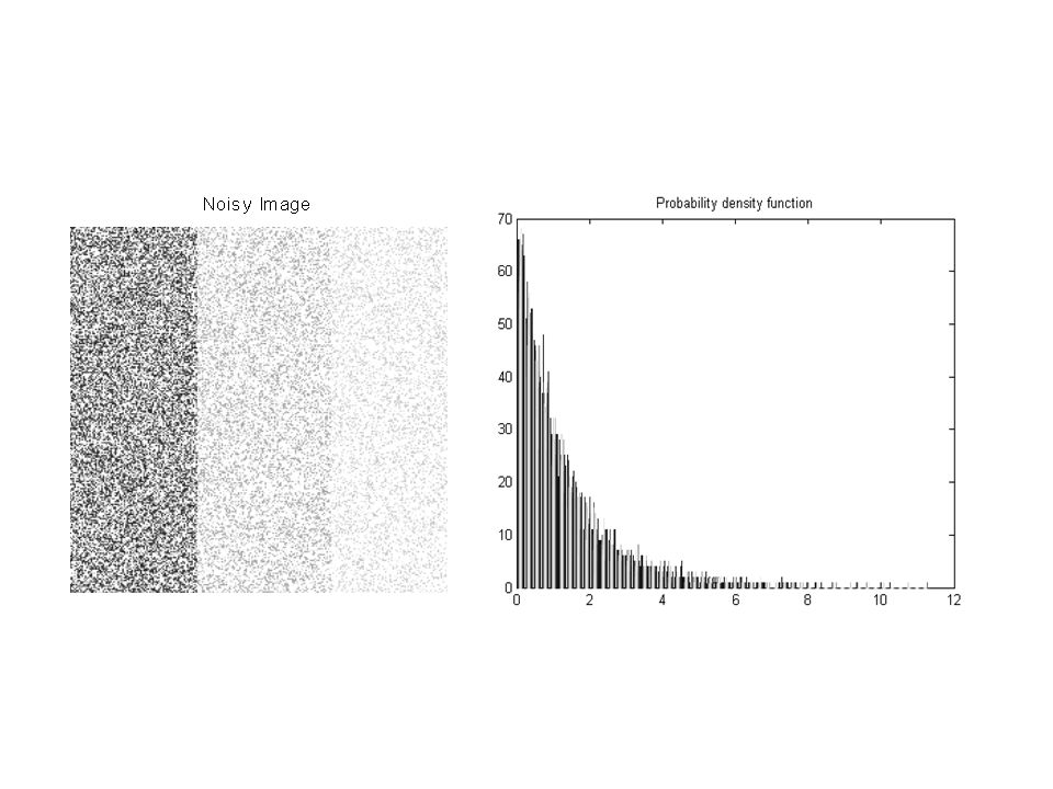
7. Noise Probability Density Functions The noise component is considered to be a random variable and characterized by a probability density function (PDF). Some common PDFs used in image processing are: Gaussian noise Gaussian (or normal) noise wide spread in usage. The PDF of a Gaussian random variable, z is given by p(z) = (1/sqrt(2*Л*σ)).exp (-(z-μ) 2 /2* σ 2 ) Here z represents gray level, μ is the mean of z, and σ is the standard deviation. The square of standard deviation is called the variance of z. Nearly 70% of the value of this function lies in the range [(μ – σ), (μ + σ)] and about 95% of its value lies in the range [(μ –2 σ), (μ + 2σ)].

9. % Gaussian noise % Read a gray scale image (having few regulat patterns) and add gaussian % noise of certain mean value,standard deviation and certain percentage. % plot the histogram of noise, noisy image. ensure that the profile of the % noise is visible in the profile of the noisy image. clear all; close all; clc; a = imread('pattern.png'); a = im2double(a); sizeA = size(a); p3 = 0; % Gaussian noise mean value p4 = 1; % Gaussian noise variance value R = p3+p4*randn([256,256]); R1 = a+R; figure,imshow(R1),title('Noisy Image'); figure,hist(R,50),title('Probability density function');

10. Rayleigh noise The PDF of Rayleigh noise is given by p(z) = (2/b)*(z-a)*exp(-(z-a) 2 /bfor z ≥ a = 0for z < a The mean and variance of this PDF are: μ = a + sqrt(Πb/4) and σ 2 = b(r – Π)/4. One has to note the displacement of PDF from the origin and skewed to the right. Thus this is useful for skewed histograms.

12. % Rayleigh noise % Read a gray scale image (having few regulat patterns) and add rayleigh % noise of certain mean value,standard deviation and certain percentage. % plot the histogram of noise, noisy image. ensure that the profile of the % noise is visible in the profile of the noisy image. clear all; close all; clc; a = imread('pattern.png'); a = im2double(a); sizeA = size(a); p3 = 0.95; A = 0; B = 2; R = A + (-B*log(1-rand(sizeA))).^0.5; x = rand(sizeA); b=a; for i=1:sizeA(1) for j=1:sizeA(2) if (x(i,j)< p3) b(i,j)=a(i,j)+R(i,j); end figure,imshow(a); figure,imshow(b),title('Noisy Image'); figure,hist(R,50),title('Probability density function'); figure,hist(b);

13. Erlang (Gamma) noise The PDF of Erlang noise is given by a b z b-1 p(z) = -------- e -az for z ≥ 0 (b -1) ! = 0for z < 0 Here a > 0, b is a positive integer. The mean and variance of this density are: μ = (b/a)andσ 2 = (b/a 2 ).

15. % erlang noise % Read a gray scale image (having few regulat patterns) and add erlang % noise of certain mean value,standard deviation and certain percentage. % plot the histogram of noise, noisy image. ensure that the profile of the % noise is visible in the profile of the noisy image. clear all; close all; clc; a = imread('pattern.png'); a = im2double(a); sizeA = size(a); p3 = 0.9; A = 2; B = 5; k = -1/A; R = zeros(sizeA); for i=1:B R = R+k*log(1-rand(sizeA)); end x = rand(sizeA); b=a; for i=1:sizeA(1) for j=1:sizeA(2) if (x(i,j)< p3) b(i,j)=a(i,j)+R(i,j); end figure,imshow(a); figure,imshow(b),title('Noisy Image'); figure,hist(R,50),title('Probability density function'); figure,hist(b);

16. Exponential noise The PDF of exponential noise is given as: p(z) = ae -az for z ≥ 0 = 0for z < 0 Here a > 0. The mean and variance of this density function are μ = (1/a)andσ 2 = (1/a 2 ). This PDF is the special case of the Erlang PDF, with b =1.

18. % Exponential noise % Read a gray scale image (having few regulat patterns) and add exponential % noise of certain mean value,standard deviation and certain percentage. % plot the histogram of noise, noisy image. ensure that the profile of the % noise is visible in the profile of the noisy image. clear all; close all; clc; a = imread('pattern.png'); a = im2double(a); sizeA = size(a); p3 = 0.9; A = 1; k = -1/A; R = k*log(1-rand(sizeA)); x = rand(sizeA); b=a; for i=1:sizeA(1) for j=1:sizeA(2) if (x(i,j)< p3) b(i,j)=a(i,j)+R(i,j); end figure,imshow(a); figure,imshow(b),title('Noisy Image'); figure,hist(R,50),title('Probability density function'); figure,hist(b);

19. Uniform noise The PDF of uniform noise is given by: p(z) = (1/(b-a))if a ≤ z ≤ b = 0otherwise The mean and variance are given as: μ = (a+b)/2andσ 2 = ((b-a) 2 )/12.

21. % Uniform noise % Read a gray scale image (having few regulat patterns) and add uniform % noise of certain mean value,standard deviation and certain percentage. % plot the histogram of noise, noisy image. ensure that the profile of the % noise is visible in the profile of the noisy image. clear all; close all; clc; a = imread('pattern.png'); %a = zeros([256,256]); a = im2double(a); sizeA = size(a); A = 0; % Min noise level B = 1; % Max noise level p3 = 0.95; % Noise percentage R = A + (B - A)*rand(sizeA); x = rand(sizeA); b=a; for i=1:sizeA(1) for j=1:sizeA(2) if x(i,j) < p3 b(i,j)=a(i,j)+R(i,j); end end figure,imshow(a); figure,imshow(b),title('Noisy Image'); figure,hist(R,50),title('Probability density function'); figure,hist(b);

22. Impulse ( salt and pepper) noise The PDF of (bipolar) impulse noise is given by: p(z) = P a for z = a = P b for z = b = 0otherwise If b > a, gray-level b will appear as a light dot in the image. Level a will appear like a dark dot. If either P a or P b is zero, the impulse noise is called unipolar. If both the probabilities are equal, impulse noise will resemble salt and pepper noise. Hence bipolar noise is also called as salt-and- pepper noise or Shot and spike noise.

23. Impulse Noise Noise impulses can be positive or negative. Generally impulse corruption is large compared to the strength of image signal and hence are treated as extreme (black or white) values. Negative impulses appear s black (pepper) points. Positive impulses appear white (salt) noise. For an 8 bit image a = 0 (black) and b = 255 (white).

25. % Salt & pepper noise noise % Read a gray scale image (having few regulat patterns) and add salt & % pepper noise of certain mean value,standard deviation and certain percentage. % plot the histogram of noise, noisy image. ensure that the profile of the % noise is visible in the profile of the noisy image. clear all; close all; clc; %a = imread('pattern.png'); a = zeros([256,256]); a = im2double(a); sizeA = size(a); p3 = 0.3; b = a; x = rand(sizeA); b(x < p3/2) = 0; % Minimum value b(x >= p3/2 & x < p3) = 1; % Maximum (saturated) value figure,imshow(a); figure,imshow(b),title('Noisy Image'); figure,hist(b,50),title('Probability density function');

26. Origin of Noises Gaussian noise arises in an image such as electronic circuit noise and sensor noise due to poor illumination and/or high temperature. The Rayleigh noise arises in range imaging. The exponential and gamma noises appear in laser imaging. Impulse noise is found in places where quick transients, such as faulty switching take place during imaging.

27. Restoring Noisy images in spatial domain Spatial filtering is good when only additive noise is present. Arithmetic mean filter Let S xy represent the set of coordinates in a rectangular subimage window of size m X n, centered at (x,y). The arithmetic mean filter computes the average value of the corrupted image g(x,y) in the area of S xy. The restored image f’ at any point (x,y) is the arithmetic mean calculated using the region of S xy. Thus, f’(x,y) = (1/mn) * Σ g(s,t) This operation is carried on a convolution mask in which all coefficients have the value (1/mn). This filter simply smoothes local variations in an image. Noise is reduce as a result of blurring.

28. Geometric mean filter This filter can be implemented using the expression: f’(x,y) = [ Π g(s,t) ] 1/mn Here each restored pixel is given by the product of the pixels in the subimage window, raised to the power of 1/mn. It gives smoothing comparable to that of arithmetic mean filter, but tends to lose less image detail during the process.

30. Harmonic mean filter This filter can be given by: f’(x,y) = (mn) / Σ (1/g(s,t)). This filter is good for removing salt noise. But fails to remove pepper noise. It works well with other noises such as Gaussian noise.

32. % Harmonic mean filter % Read a gray scale image and add a noise to it and filter it using % Harmonic mean filter. clear all; close all; clc; f = imread('Saltcman.tif'); %f = imnoise(f,'gaussian',0,0.02); f = im2double(f); %subplot(1,2,1),imshow(f),title('Original Image'); figure,imshow(f),title('Salt Noise'); [m n]=size(f); for i = 2:m-1 for j = 2:n-1 con=0; s1=0; for k1 = i-1:i+1 for p1 = j-1:j+1 con = con+1; if f(k1,p1)==0 s1 = s1+0; else s1=s1+(1/f(k1,p1)); end b1(i,j)=con/s1; end %subplot(1,2,2),imshow(b1),title('Harmonic mean filtered'); figure,imshow(b1),title('Harmonic mean filtered');

33. Contra harmonic mean filter This filer can be implemented using the expression: f’(x,y) = Σ g(s,t) Q+1 /Σ g(s,t) Q Here Q is the order of the filter. It is good for reducing the effect of salt and pepper noise. For positive values of Q, it eliminates pepper noise and for negative values of Q it eliminates salt noise. It reduces to arithmetic mean filter for Q = 0 and harmonic mean filter for Q = -1. Generally, the positive order filter cleans the background, by blurring dark areas.

34. Contra harmonic mean filter Arithmetic and geometric mean filters are good for removing random noise like Gaussian or uniform noise. Contraharmonic filer is good for impulse noise. But it must be known before hand that whether the noise is dark or light to fix the Q value.

36. % Contraharmonic mean filter % Read a gray scale image and applay contraharmonic filter for verious Q % values. prove that for negative values of Q salt noise is removed, for % positive values of Q pepper noise is removed. check that % for Q=0 it becomes mean filter and for Q=-1 it becomes harmonic filter. clear all; close all; clc; f = imread('Peppercman.tif'); %f = imnoise(f,'salt & pepper',0.1); f = im2double(f); %subplot(1,2,1),imshow(f),title('Original Image'); figure,imshow(f),title('Pepper Noise'); [m n]=size(f); Q=1; for i = 2:m-1 for j = 2:n-1 con=0; s1=0; s2=0; for k1 = i-1:i+1 for p1 = j-1:j+1 con = con+1; s1=s1+(f(k1,p1)^Q); s2=s2+(f(k1,p1)^(Q+1)); end b1(i,j)=s2/s1; end %subplot(1,2,2),imshow(b1),title('Cantraharmonic mean filtered'); figure,imshow(b1),title('Contraharmonic mean filtered ');

37. Order Statistics Filter These are spatial filters whose response is based on ordering (ranking) the pixels in the image area encompassed by the filter. Median filter Here we replace the value of a pixel by the median of the gray values in the neighborhood of that pixel: f’(x,y) = median {g(s,t)} The original value of the pixel is included in the calculation of the median. For some types of random noise, they give excellent noise-reduction with less blurring than linear smoothing filters of same size. They work well with unipolar and bipolar impulse noises.

39. Max and min filters Median is the 50 th percentile of a ranked set of numbers. The 100 th percentile results in max filter given as: f’(x,y) = max {g(s,t)} This filter is useful in finding the brightest spots in an image. As pepper noise has very low intensity values, they are reduced by this filter. The 0 th percentile filter is the min filter: f’(x,y) = min {g(s,t)} this filter is capable of identifying the darkest points in an image. It reducecs salt noise as a result of min operation.

42. % Max and Min filters % Read a gray scale image and add salt & pepper noise and remove the same % with min filter and max filter. clear all; close all; clc; f = imread('cameraman.tif'); f = imnoise(f,'salt & pepper',0.01); f = im2double(f); %subplot(2,2,1),imshow(f),title('Original Image'); figure,imshow(f),title('Noisy Image'); [m n]=size(f); Q=0; for i = 2:m-1 for j = 1:n-1 con=0; for k1 = i-1:i+1 for p1 = j-1:j+1 con = con+1; s1(con)=(f(k1,p1)); end b1(i,j)=min(s1); b2(i,j)=max(s1); end %subplot(2,2,2),imshow(b1),title('Min filter'); %subplot(2,2,3),imshow(b2),title('Max filter'); figure,imshow(b1),title('Min filter'); figure,imshow(b2),title('Max filter');

43. Midpoint filter This filter is simply the midpoint between the maximum and minimum values in the area enclosed by the filter: f’(x,y) = (1/2) * [ max {g(s,t)} + min {g(s,t)}] This filter combines order statistic and averaging. It is good for randomly distributed noise, like Gaussian or uniform noise.

45. % Midpoint filter % Read a gray scale image and add gaussian noise and remove the noise using % midpoint filter clear all; close all; clc; f = imread('cameraman.tif'); f = imnoise(f,'gaussian',0,0.01); f = im2double(f); %subplot(1,2,1),imshow(f),title('Noisy Image'); figure,imshow(f),title('Noisy Image'); [m n]=size(f); Q=0; for i = 2:m-1 for j = 2:n-1 con=0; for k1 = i-1:i+1 for p1 = j-1:j+1 con = con+1; s1(con)=(f(k1,p1)); end b1=min(s1); b2=max(s1); R_img(i,j)=(b1+b2)/2; end %subplot(1,2,2),imshow(R_img),title('Midpoint filtered'); figure,imshow(R_img),title('Midpoint filtered');

46. Alpha trimmed mean filter Let us delete the d/2 lowest and the d/2 highest gray-level values of g(s,t) in the neighborhood of S xy. Let g r (s,t) represent the remaining (mn – d ) pixels. A filter formed by averaging these remaining pixels is called an alpha-trimmed mean filter: f’(x,y) = (1/(mn-d))* Σ g r (s,t) Here the value of d can vary from 0 to (mn – 1). When d = 0, it reduces to arithmetic mean filter. For d = (mn-1)/2, it becomes a median filter. For other values of d, it is useful in situations involving multiple types of noise, such as combination of salt and pepper and Gaussian noise.

48. % read a gray scale image and remove the salt & pepper noise using alpha % trimed mean filter. prove that for D=0 it becomes arithmetic mean filter % and for d=(mn-1)/2 it becomes median filter. show that this filter % removes combination of gaussian and salt & pepper noise. clear all; close all; clc; f = imread('cameraman.tif'); f = im2double(f); f = imnoise(f,'salt & pepper',0.1); f = imnoise(f,'gaussian',0,0.01); [m n]=size(f); f1=zeros(m,n); D = 4; d = D/2; for i=3:m-2 for j=3:n-2 con=0; for k=i-2:i+2 for p=j-2:j+2 con=con+1; s(con)=f(k,p); end s = sort(s); r = (size(s,2)-d); s1= s(d+1:r); f1(i,j)= sum(s1)/(con-D); end figure,imshow(f),title('Noisy Image'); figure,imshow(f1),title('Alpha-trimmed mean filter');

49. Adaptive filters The filters discussed above, do not worry about the image characteristics. Adaptive filters are one whose behavior changes based on statistical characteristics of the image inside the filter region defined by the m X n subimage. Adaptive, local noise reduction filter Mean and variance are the simple statistical feature of a random variable. They are related to the appearance of an image. Mean gives a measure of average gray level in the region over which the mean is computed and variance gives a measure of average contrast in that region.

50. Response of a filter The response of a filter at (x,y) depends on: g(x,y), the value of the noisy image at (x,y). σ η 2, the variance of the noise corrupting the image f(x,y) m L, the local mean of the pixels in S xy. σ L 2, the local variance of the pixels in S xy.

51. Behavior of a filter The filter should behave as follows: If σ η 2 is zero, filter should return the value of g(x,y). If local variance is high relative to σ η 2, the filter should return a value close to g(x,y). A high local variance is related with edges, and should be preserved. If the 2 variances are equal, the filter should return the arithmetic mean value of the pixels in S xy.

52. Behavior of a filter An adaptive expression for obtaining f’(x,y) based on these assumptions is given as: f’(x,y) = g(x,y) – (σ η 2 / σ L 2 ) * [g(x,y) – m L ] One needs to know or estimate the variance of overall noise σ η 2. Other parameters are calculated from the pixels in S xy. A general assumption is that σ η 2 ≤ σ L 2. This is true because we assume that our noise is additive and position independent as the subimge is the subset of g(x,y).

53. Behavior of a filter Here if the estimate of σ η 2 is too low, then the algorithm will return an image that resembles the original image as the correction factors are too small. If the estimates are too high, the ratio of the variances need to be clipped at 1.0 and the algorithm will subtract the man from the image more frequently than it would normally do so. If negative values are permitted, the image is rescaled at the end and the result is a loss of dynamic range.

55. % Read a gray scale image and add gaussian noise with 0 mean then apply % the Adaptive local noise reduction filter. clear all; close all; clc; f = imread('cameraman.tif'); f = im2double(f); [m n]=size(f); f1=zeros(m,n); f = imnoise(f,'gaussian',0,0.1); D = std2(f); M = mean2(f); for i=3:m-2 for j=3:n-2 con=0; s=0; s1=0; for k=i-2:i+2 for p=j-2:j+2 con=con+1; s = s+f(k,p); s1(con)=f(k,p); end lm=s/con; ld = std(s1); if ld >0 f1(i,j) = f(i,j)-((D*(f(i,j)-lm)/ld)); else f1(i,j) = f(i,j)-0; end figure,imshow(f),title('Gaussian Noise Image'); figure,imshow(f1),title('Adaptive Local Noise Filtered');

56. Adaptive median filter The median filter works well if the spatial density of impulse noise is not large (if P a and P b are less than 0.2). But adaptive median filters can handle impulse noises of greater strength. Adaptive median filter preserve the detail while smoothing nonimpulse noise, which is not done by normal median filter. The adaptive median filter changes (increases) the size of S xy during the filter operation. The output of a median filter is a single value replacing the value of the pixel at (x,y), the point at which the window is centered.

57. Adaptive median filter Let z min, z max = minimum and maximum gray level value in S xy z med = median of gray level value in S xy z xy = gray level at coordinates (x,y) S max = maximum allowed size of S xy

58. Working of adaptive median filter The adaptive median filter works in 2 levels, called as level A and level B. Level A : A1 = z med - z min A2 = z med – z max If A1 > 0 AND A2 < 0, Go to level B Else increase the window size If window size ≤ S max repeat level A Else output z xy. Level B :B1 = z xy - z min B2 = z xy – z max If B1 > 0 AND B2 < 0, output zxy. Else output z med.

59. Working of adaptive median filter This algorithm does 3 things: Removes slat and pepper noise (impulse noise) Smoothing other non-impulsive noises. Reduce distortion such as excessive thinning or thickening of object boundaries. The purpose of level A is to find if the median filter output, z med is an impulse (black and white) or not. If the condition z min < z med < z max holds, then z med cannot be an impulse noise.

60. Working of adaptive median filter Now we go to level B and test whether the center pixel z xy itself is an impulse. If B1 > 0 AND B2 < 0 is true, then z min < z xy < z max and z xy cannot be an impulse. Now the output of the algorithm is unchanged pixel value z xy. By not changing these “intermediate level” points, distortion is reduced in the image. If the condition B1 > 0 AND B2 < 0 is false, then either z xy = z min or z xy = z max. In both the cases, the value of the pixel is an extreme value and the algorithm outputs the median value z med which we know from level A is not a noise impulse.