1. Frequency Analysis Professor Ke-Sheng Cheng
Dept. of Bioenvironmental Systems Engineering
National Taiwan University

2. General interpretation of hydrological frequency analysis
Hydrological frequency analysis is the work of determining the magnitude of hydrological variables that corresponds to a given probability of exceedance. Frequency analysis can be conducted for many hydrological variables including floods, rainfalls, and droughts.
The work can be better perceived by treating the interested variable as a random variable.

3. Let X represent the hydrological (random) variable under investigation
Let X represent the hydrological (random) variable under investigation. A value xc associating to some event is chosen such that if X assumes a value exceeding xc the event is said to occur. Every time when a random experiment (or a trial) is conducted the event may or may not occur.
We are interested in the number of Bernoulli trials in which the first success occur. This can be described by the geometric distribution.

4. Geometric distribution
Geometric distribution represents the probability of obtaining the first success in x independent and identical Bernoulli trials.

6. Recurrence interval vs return period
Average number of trials to achieve the first success.
Recurrence interval vs return period

8. The frequency factor equation

10. It is apparent that calculation of involves determining the type of distribution for X and estimation of its mean and standard deviation. The former can be done by GOF test and the latter is accomplished by parametric point estimation.
Collecting required data.
Determining appropriate distribution.
Estimating the mean and standard deviation.
Calculating xT using the general eq.

11. Data series used for frequency analysis
Complete duration series
A complete duration series consists of all the observed data.
Partial duration series
A partial duration series is a series of data which are selected so that their magnitude is greater than a predefined base value. If the base value is selected so that the number of values in the series is equal to the number of years of the record, the series is called an “annual exceedance series”.

12. Extreme value series Data independency
An extreme value series is a data series that includes the largest or smallest values occurring in each of the equally-long time intervals of the record. If the time interval is taken as one year and the largest values are used, then we have an “annual maximum series”.
Data independency
Why is it important?

13. Techniques for goodness-of-fit test
A good reference for detailed discussion about GOF test is:
Goodness-of-fit Techniques. Edited by R.B. D’Agostino and M.A. Stephens, 1986.
Probability plotting
Chi-square test
Kolmogorov-Smirnov Test
Moment-ratios diagram method
L-moments based GOF tests

14. Rainfall frequency analysis
Consider event total rainfall at a location.
What is a storm event?
Parameters related to partition of storm events
Minimum inter-event-time
A threshold value for rainfall depth

16. Total depths of storm events
Total rainfall depth of a storm event varies with its storm duration. [A bivariate distribution for (D, tr).]
For a given storm duration tr, the total depth D(tr) is considered as a random variable and its magnitudes corresponding to specific exceedance probabilities are estimated. [Conditional distribution]
In general,

17. Probabilistic Interpretation of the Design Storm Depth

18. Random Sample For Estimation of Design Storm Depth
The design storm depth of a specified duration with return period T is the value of D(tr) with the probability of exceedance equals  /T.
Estimation of the design storm depth requires collecting a random sample of size n, i.e., {x1, x2, …, xn}.
A random sample is a collection of independently observed and identically distributed (IID) data.

19. Annual Maximum Series
Data in an annual maximum series are considered IID and therefore form a random sample.
For a given design duration tr, we continuously move a window of size tr along the time axis and select the maximum total values within the window in each year.
Determination of the annual maximum rainfall is NOT based on the real storm duration; instead, a design duration which is artificially picked is used for this purpose.

20. Fitting A Probability Distribution to Annual Maximum Series
How do we fit a probability distribution to a random sample?
What type of distribution should be adopted?
What are the parameter values for the distribution?
How good is our fit?

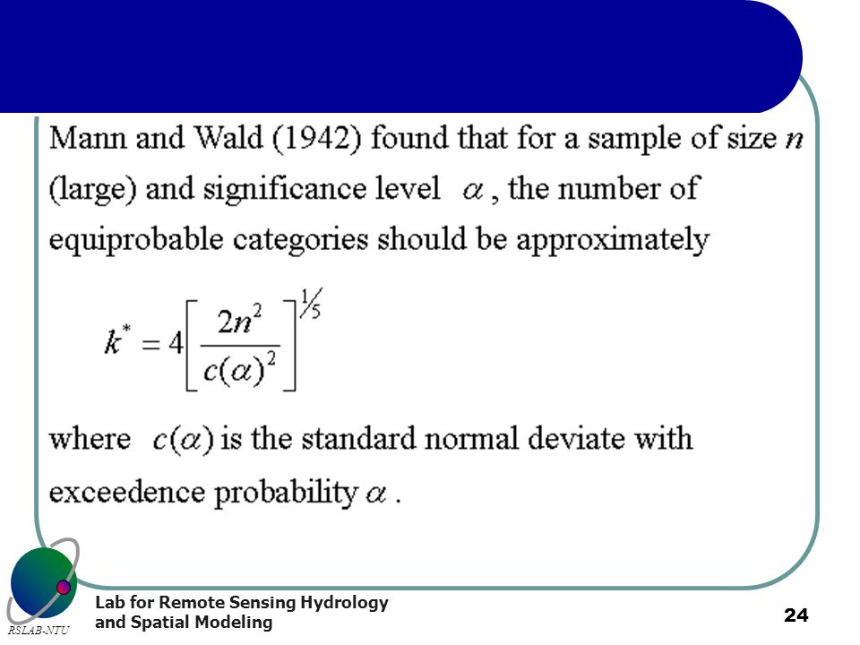
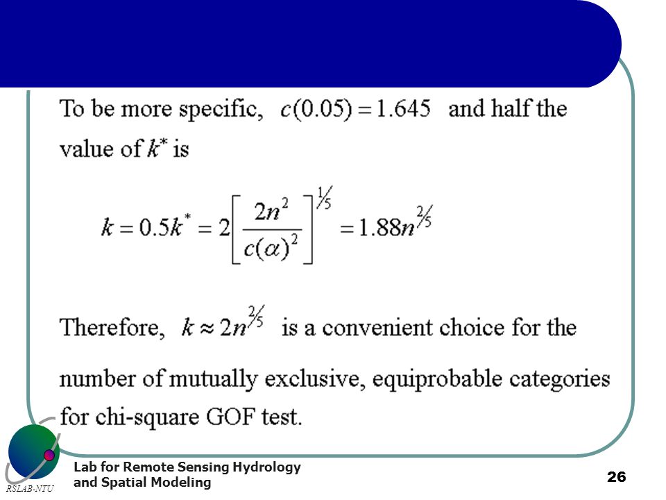
21. Chi-square GOF test

28. Kolmogorov-Smirnov GOF test
The chi-square test compares the empirical histogram against the theoretical histogram.
In contrast, the K-S test compares the empirical cumulative distribution function (ECDF) against the theoretical CDF.

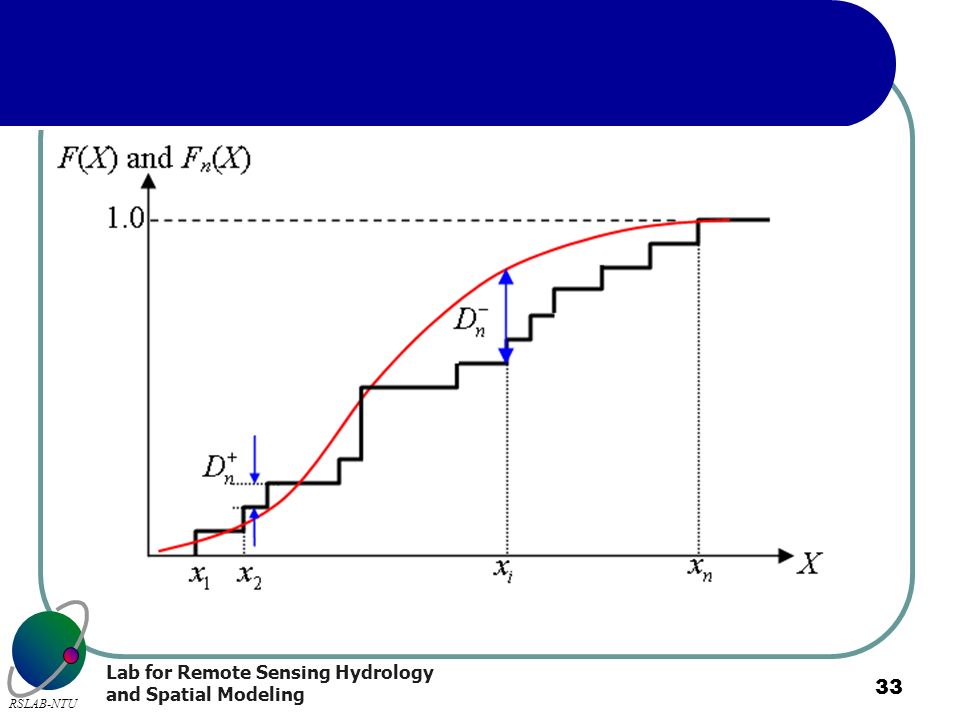
32. In order to measure the difference between Fn(X) and F(X), ECDF statistics based on the vertical distances between Fn(X) and F(X) have been proposed.

38. Hypothesis test using Dn

39. Values of for the Kolmogorov-Smirnov test

40. GOF test using L-moment-ratios diagram (LMRD)
Concept of identifying appropriate distributions using moment-ratio diagrams (MRD).
Product-moment-ratio diagram (PMRD)
L-moment-ratio diagram (LMRD)
Two-parameter distributions
Normal, Gumbel (EV-1), etc.
Three-parameter distributions
Log-normal, Pearson type III, GEV, etc.

41. Moment ratios are unique properties of probability distributions and sample moment ratios of ordinary skewness and kurtosis have been used for selection of probability distribution.
The L-moments uniquely define the distribution if the mean of the distribution exists, and the L-skewness and L-kurtosis are much less biased than the ordinary skewness and kurtosis.

42. A two-parameter distribution with a location and a scale parameter plots as a single point on the LMRD, whereas a three-parameter distribution with location, scale and shape parameters plots as a curve on the LMRD, and distributions with more than one shape parameter generally are associated with regions on the diagram.
However, theoretical points or curves of various probability distributions on the LMRD cannot accommodate for uncertainties induced by parameter estimation using random samples.

43. Ordinary (or product) moment-ratios diagram (PMRD)

44. The ordinary (or product) moment ratios diagram

46. Sample estimates of product moment ratios

48. (D'Agostino and Stephens, 1986)
95％
90％

49. Even though joint distribution of the ordinary sample skewness and sample kurtosis is asymptotically normal, such asymptotic property is a poor approximation in small and moderately samples, particularly when the underlying distribution is even moderately skew.

51. Scattering of sample moment ratios of the normal distribution
(100,000 random samples)

52. L-moments and the L-moment ratios diagram

56. L-moment-ratio diagram of various distributions

57. Sample estimates of L-moment ratios (probability weighted moment estimators)

59. Sample estimates of L-moment ratios (plotting-position estimators)

60. Hosking and Wallis (1997) indicated that is not an unbiased estimator of , but its bias tends to zero in large samples.
and are respectively referred to as the probability-weighted-moment estimator and the plotting-position estimator of the L-moment ratio .

61. Establishing acceptance region for L-moment ratios
The standard normal and standard Gumbel distributions (zero mean and unit standard deviation) are used to exemplify the approach for construction of acceptance regions for L-moment ratio diagram.
L-moment-ratios ( , ) of the normal and Gumbel distributions are respectively (0, ) and (0.1699, ).

62. Stochastic simulation of the normal and Gumbel distributions
For either of the standard normal and standard Gumbel distribution, a total of 100,000 random samples were generated with respect to the specified sample size20, 30, 40, 50, 60, 75, 100, 150, 250, 500, and 1,000.
For each of the 100,000 samples, sample L-skewness and L-kurtosis were calculated using the probability-weighted-moment estimator and the plotting-position estimator.

63. Scattering of sample L-moment ratios Normal distribution
(100,000 random samples)

64. Normal distribution ?
(100,000 random samples)

65. Non-normal distribution !
95% acceptance region
99% acceptance region
Non-normal distribution !
(100,000 random samples)

66. Scattering of sample L-moment ratios Gumbel distribution
(100,000 random samples)

67. (100,000 random samples)

68. (100,000 random samples)

69. For both distribution types, the joint distribution of sample L-skewness and L-kurtosis seem to resemble a bivariate normal distribution for a larger sample size (n = 100).
However, for sample size n = 20, the joint distribution of sample L-skewness and L-kurtosis seems to differ from the bivariate normal. Particularly for Gumbel distribution, sample L-moments of both estimators are positively skewed.

70. For smaller sample sizes (n = 20 and 50), the distribution cloud of sample L-moment-ratios estimated by the plotting-position method appears to have its center located away from ( , ), an indication of biased estimation.
However, for sample size n = 100, the bias is almost unnoticeable, suggesting that the bias in L-moment-ratio estimation using the plotting-position estimator is negligible for larger sample sizes.

71. In contrast, the distribution cloud of the sample L-moment-ratios estimated by the probability-weighted-moment method appears to have its center almost coincide with ( , ).

72. Bias of sample L-skewness and L-kurtosis - Normal distribution

74. Bias of sample L-skewness and L-kurtosis - Gumbel distribution

76. Mardia test for bivariate normality of sample L-skewness and L-kurtosis

80. Mardia test for bivariate normality of sample L-skewness and L-kurtosis

81. Mardia test for bivariate normality of sample L-skewness and L-kurtosis

82. It appears that the assumption of bivariate normal distribution for sample L-skewness and L-kurtosis of both distributions is valid for moderate to large sample sizes. However, for random samples of normal distribution with sample size , the bivariate normal assumption may not be adequate. Similarly, the bivariate normal assumption for sample L-skewness and L-kurtosis of the Gumbel distribution may not be adequate for sample size

83. Establishing acceptance regions for LMRD-based GOF tests
For moderate to large sample sizes, the sample L-skewness and L-kurtosis of both the normal and Gumbel distributions have asymptotic bivariate normal distributions.
Using this property, the acceptance region of a GOF test based on sample L-skewness and L-kurtosis can be determined by the equiprobable density contour of the bivariate normal distribution with its encompassing area equivalent to

84. The probability density function of a multivariate normal distribution is generally expressed by
The probability density function depends on the random vector X only through the quadratic form which has a chi-square distribution with p degrees of freedom.

85. Therefore, probability density contours of a multivariate normal distribution can be expressed by
for any constant
For a bivariate normal distribution (p=2) the above equation represents an equiprobable ellipse, and a set of equiprobable ellipses can be constructed by assigning to c for various values of .

86. Consequently, the acceptance region of a GOF test based on the sample L-skewness and L-kurtosis is expressed by
where is the upper quantile of the distribution at significance level .

87. For bivariate normal random vector , the density contour of can also be expressed as
However, the expected values and covariance matrix of sample L-skewness and L-kurtosis are unknown and can only be estimated from random samples generated by stochastic simulation.

88. Thus, in construction of the equiprobable ellipses, population parameters must be respectively replaced by their sample estimates
The Hotelling’s T2 statistic

89. The Hotelling’s T2 is distributed as a multiple of an F-distribution, i.e.,
For large N,
Therefore, the distribution of the Hotelling’s T2 can be well approximated by the chi-square distribution with degree of freedom 2.

90. Thus, if the sample L-moments of a random sample of size n falls outside of the corresponding ellipse, i.e.
the null hypothesis that the random sample is originated from a normal or Gumbel distribution is rejected.

91. Scattering of sample L-moment ratios Normal distribution
(100,000 random samples)

92. Normal distribution ?
(100,000 random samples)

93. Variation of 95% acceptance regions with respect to sample size n
Non-normal distribution !
What if n=36?
(100,000 random samples)

94. Empirical relationships between parameters of acceptance regions and sample size
Since the 95% acceptance regions of the proposed GOF tests are dependent on the sample size n, it is therefore worthy to investigate the feasibility of establishing empirical relationships between the 95% acceptance region and the sample size. Such empirical relationships can be established using the following regression model

95. Empirical relationships between the sample size and parameters of the bivariate distribution of sample L-skewness and L-kurtosis

96. Empirical relationships between the sample size and parameters of the bivariate distribution of sample L-skewness and L-kurtosis

97. Example
Suppose that a random sample of size n = 44 is available, and the plotting-position sample L-skewness and L-kurtosis are calculated as ( , ) = (0.214, 0.116). We want to test whether the sample is originated from the Gumbel distribution.

98. From the regression models for plotting-position estimators, we find
to be respectively , , , , and The Hotelling’s T2 is then calculated as
The value of T2 is much smaller than the threshold value

99. The null hypothesis that the random sample is originated from the Gumbel distribution is not rejected.

100. 95% acceptance regions of L-moments-based GOF test for the normal distribution
Acceptance ellipses correspond to various sample sizes (n = 20, 30, 40, 50, 60, 75, 100, 150, 250, 500, and 1,000).

101. Acceptance ellipses correspond to various sample sizes (n = 20, 30, 40, 50, 60, 75, 100, 150, 250, 500, and 1,000).

102. 95% acceptance regions of L-moments-based GOF test for the Gumbel distribution
Acceptance ellipses correspond to various sample sizes (n = 20, 30, 40, 50, 60, 75, 100, 150, 250, 500, and 1,000).

103. Acceptance ellipses correspond to various sample sizes (n = 20, 30, 40, 50, 60, 75, 100, 150, 250, 500, and 1,000).

104. Validity check of the LMRD acceptance regions
The sample-size-dependent confidence intervals established using empirical relationships described in the last section are further checked for their validity. This is done by stochastically generating 10,000 random samples for both the standard normal and Gumbel distributions, with sample size20, 30, 40, 50, 60, 75, 100, 150, 250, 500, and 1,000.

106. For validity of the sample-size-dependent 95% acceptance regions, the rejection rate should be very close to the level of significance ( ) or the acceptance rate be very close to 0.95.

107. Acceptance rate of the validity check for sample-size-dependent 95% acceptance regions of sample L-skewness and L-kurtosis pairs.
Based on 10,000 random samples for any given sample size n.

108. End of this session.