1. 1. The Simplex Method

2. Restaurant owner problem
max 8x + 6y
Subject to
5x + 3y ≤ 30
2x + 3y ≤ 24
1x + 3y ≤ 18
x,y ≥ 0
Seafoods available:
30 sea-urchins
24 shrimps
18 oysters
Two types of seafood plates to be offered:
$8 : including 5 sea-urchins, 2 shrimps et 1 oyster
$6 : including 3 sea-urchins, 3 shrimps et 3 oysters
Problem: determine the number of each type of plates to be offered by the
owner in order to maximize his revenue according to the seafoods
available

3. Transforming max problem into min problem
Consider the following maximisation problem
max f(w)
Subject to
where f : X → R1.
Let w* be a point of X where the maximum of f is reached.
Then f(w*) ≥ f(w)
or – f(w*) ≤ – f(w)
Consequently
– f(w*) = min – f(w)
Subject to w X Rn
and w* is a point of X where the function – f(w) reaches its minimum.
Hence if we max f(w) or if we min – f(w) we find the same optimal
solution w* .

4. f(w*)
f(w) w w*
– f(w)
– f(w*)

5. Transforming max problem into min problem
Furthermore
f(w*) = max f(w) = – min – f(w) = – (–f(w*) )
We will always transform max problem into min problem.
Then f(w*) ≥ f(w)
or – f(w*) ≤ – f(w)
Consequently
– f(w*) = min – f(w)
Subject to w X Rn
and w* is a point of X where the function – f(w) reaches its minimum.
Hence if we max f(w) or if we min – f(w) we find the same optimal
solution w* .

6. Restaurant owner problem
max 8x + 6y
Subject to
5x + 3y ≤ 30
2x + 3y ≤ 24
1x + 3y ≤ 18
x,y ≥ 0
min – (8x + 6y)
Subject to
5x + 3y ≤ 30
2x + 3y ≤ 24
1x + 3y ≤ 18
x,y ≥ 0

7. Solving a problem graphically
Method to solve problem having only two variables
Consider the restaurant owner problem transformed into a min problem:
min z = –8x – 6y
Subject to
5x + 3y ≤ 30
2x + 3y ≤ 24
1x + 3y ≤ 18
x,y ≥ 0

8. Feasible Domain Draw the line 5x + 3y = 30
The set of points satisfying
the constraint
5x + 3y ≤ 30
is under the line since the origin
satisfies the constraint

9. Feasible Domain Draw the line 2x + 3y = 24
The set of points satisfying
the constraint
2x + 3y ≤ 24
is under the line since the origin
satisfies the constraint

10. Feasible Domain Draw the line x + 3y = 18 The set of points satisfying
the constraint
x + 3y ≤18
is under the line since the origin
satisfies the constraint

11. Feasible Domain The set of feasible points for the system 5x + 3y ≤ 30

12. Solving the problem Consider the economic function : z = –8x – 6y.
The more we move away on the right of the origin, the more the objective function decreases:
x = 0 and y = 0 => z = 0

13. Solving the problem Consider the economic function : z = –8x – 6y.
The more we move away on the right of the origin, the more the objective function decreases:
x = 0 and y = 0 => z = 0
x = 0 and y = 6 => z = – 36

14. Solving the problem Consider the economic function : z = –8x – 6y.
The more we move away on the right of the origin, the more the objective function decreases:
x = 0 and y = 0 => z = 0
x = 0 and y = 6 => z = – 36
x = 6 and y = 0 => z = – 48

15. Solving the problem Consider the economic function : z = –8x – 6y.
The more we move away on the right of the origin, the more the objective function decreases:
x = 0 and y = 0 => z = 0
x = 0 and y = 6 => z = – 36
x = 6 and y = 0 => z = – 48
x = 3 and y = 5 => z = – 54.
Cannot move further on the right without going out of the feasible domain.
Optimal solution:
x = 3 et y = 5
Optimal value:
z = – 54

16. Slack variables
Modify an inequality constraint into an equality constraint using non negative slack variables:
ai1x1 + ai2x2 + … + ainxn ≤ bi → ai1x1 + ai2x2 + … + ainxn + yi = bi
yi ≥ 0
ai1x1 + ai2x2 + … + ainxn ≥ bi → ai1x1 + ai2x2 + … + ainxn – yi = bi

17. Minimum version of the restaurant owner
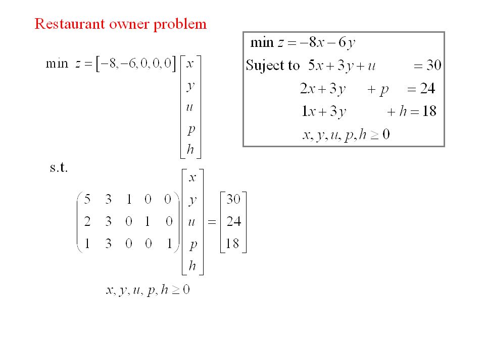
Modify the inequality constraints of the restaurant owner problem into equality constraints using the slack variables u, p, and h:
min z = – 8x – 6y min z = – 8x – 6y
s.t s.t.
5x + 3y ≤ x + 3y + u =30
2x + 3y ≤ x + 3y p =24
1x + 3y ≤ x + 3y h = 18
x, y ≥ x, y, u, p, h ≥ 0
The constraints are a linear system including 3 equations and 5 variables.
3 of the variables can be evaluated in terms of the other 2 variables

18. Dictionary Simplex Method
The constraints are a linear system including 3 equations and 5 variables.
3 of the variables can be evaluated in terms of the other 2 variables
u = 30 – 5x – 3y
p = 24 – 2x – 3y
h = 18 – 1x – 3y
z = 0 – 8x – 6y
Fixing the values of x and y induces the values of the other 3 variables.
It is sufficient to find non negatives values of x and y inducing non negatives values of u, p and h minimizing the value of z .
Infinite number of possibilities. We better have a systematic procedure to find the minimum of z.

19. Find the variable to be increased
A feasible solution of the linear system
u = 30 – 5x – 3y
p = 24 – 2x – 3y
h = 18 – 1x – 3y
z = 0 – 8x – 6y
is the following
x = y = => u = 30, p = 24, h = et z = 0.
We can reduce the value of z if we increase the value of x, or that of y, or both.
In the Simplex method we increase the value of only one
To minimize z, it seems better to increase the value of x since increasing the value of x by one unit induces reducing the value of z by 8 units.

20. Limit for increasing the variable
The non negativity of the variables u, p et h limits the increase of x
u = 30 – 5x – 3y ≥ 0
p = 24 – 2x – 3y ≥ 0
h = 18 – 1x – 3y ≥0
Since the value of y is fixed to 0, then
u = 30 – 5x ≥ 0  x ≤ 30 / 5 = 6
p = 24 – 2x ≥ 0  x ≤ 24 / 2 = 12
h = 18 – 1x ≥0  x ≤ 18
The solution remains feasible as long as
x ≤ min {6, 12, 18} = 6.

21. u = 30 – 5x – 3y New solution p = 24 – 2x – 3y h = 18 – 1x – 3y
z = 0 – 8x – 6y
The solution remains feasible as long as
x ≤ min {6, 12, 18} = 6.
In order to minimize z, we select the largest value of x:
i.e., x = 6.
The new solution becomes
x = 6, y = => u = 0, p = 12, h = et z = – 48.

22. New iteration u = 30 – 5x – 3y p = 24 – 2x – 3y h = 18 – 1x – 3y
z = 0 – 8x – 6y
The new solution becomes
x = 6, y = => u = 0, p = 12, h = et z = –48.
This solution is unique for the preceding system when y = u = 0 since the coefficients of the variables x, p et h induces a non singular matrix.
Consequently, to determine another solution, either y or u must take a positive value.
Previously, the analysis was simplified by the fact that the variables x and y that could be modified were on the right hand side.

23. Obtain an equivalent system
Modify the system to have y and u on the right hand side.
Use the equation including x et u in order to find a relation where x is a function of u and y:
u = 30 – 5x – 3y => 5x = 30 – u – 3y
p = 24 – 2x – 3y
h = 18 – 1x – 3y
z = 0 – 8x – 6y

24. Obtain an equivalent system
Modify the system to have y and u on the right hand side.
Use the equation including x et u in order to find a relation where x is a function of u and y:
u = 30 – 5x – 3y => (5x = 30 – u – 3y) ÷ 5
=> x = 6 – 1/5u – 3/5y
p = 24 – 2x – 3y
h = 18 – 1x –3y
z = 0 – 8x – 6y

25. Obtain an equivalent system
Modify the system to have y and u on the right hand side.
Use the equation including x et u in order to find a relation where x is a function of u and y:
u = 30 – 5x – 3y => x = 6 – 1/5u – 3/5y
p = 24 – 2x – 3y
=> p = 24 – 2(6 – 1/5u – 3/5y) – 3y
=> p = /5u – 9/5y
h = 18 – 1x – 3y
z = 0 – 8x – 6y
Replace x by its expression in terms of u and y in the other equations.

26. Obtain an equivalent system
Modify the system to have y and u on the right hand side.
Use the equation including x et u in order to find a relation where x is a function of u and y:
u = 30 – 5x – 3y => x = 6 – 1/5u – 3/5y
p = 24 – 2x – 3y => p = /5u – 9/5y
h = 18 – 1x – 3y
=> h = 18 – (6 – 1/5u – 3/5y) – 3y
=> h = /5u – 12/5y
z = 0 – 8x – 6y
Replace x by its expression in terms of u and y in the other equations.

27. Obtain an equivalent system
Modify the system to have y and u on the right hand side.
Use the equation including x et u in order to find a relation where x is a function of u and y:
u = 30 – 5x – 3y => x = 6 – 1/5u – 3/5y
p = 24 – 2x – 3y => p = /5u – 9/5y
h = 18 – 1x – 3y => h = /5u – 12/5y
z = 0 – 8x – 6y
=> z = 0 – 8(6 – 1/5u – 3/5y) – 6y
=> z = – /5u – 6/5y
Replace x by its expression in terms of u and y in the other equations.

28. Equivalent system We transformed the system
u = 30 – 5x – 3y => x = 6 – 1/5u – 3/5y
p = 24 – 2x – 3y => p = /5u – 9/5y
h = 18 – 1x – 3y => h = /5u – 12/5y
z = 0 – 8x – 6y => z = – /5u – 6/5y

29. Equivalent system
We have a new system equivalent to the preceding one (i.e., the two systems have the same set of feasible solutions)
Note that it is not interesting to increase u since the value of z would increase
We repeat the preceding procedure by increasing the value of y
x = 6 – 1/5u – 3/5y
p = /5u – 9/5y
h = /5u – 12/5y
z = – /5u – 6/5y

30. New iteration
The non negativity of the variables x, p et h limits the increase of y :
x = 6 – 1/5u – 3/5y ≥ 0
p = /5u – 9/5y ≥0
h = /5u – 12/5y ≥ 0
Since the value of u is fixed to 0, then
x = 6 – 3/5y ≥  y ≤ 10
p = 12 – 9/5y ≥  y ≤ 20/3
h = 12– 12/5y ≥0  y ≤ 5
The solution remains feasible as long as
y ≤ min {10, 20/3, 5} = 5.

31. New iteration x = 6 – 1/5u – 3/5y ≥ 0 p = 12 + 2/5u – 9/5y ≥0
h = /5u – 12/5y ≥ 0
z = – /5u– 6/5y
The solution remains feasible as long as
y ≤ min {10, 20/3, 5} = 5.
In order to minimize z, we select the largest value of y: : i.e., y = 5.
The new solution is
y = 5, u = => x = 3, p = 3, h = 0 et z = – 54.

32. Optimal solution
Modify the system to have h and u on the right hand side.
Use the equation including h and u in order to find a relation where y is a function of h and u:
h = /5u – 12/5y
Replace y by its expression in terms of u and y in the other equations.
The system becomes
x = 3 – 1/4u + 1/4h
p = /4u + 3/4h
y = /12u – 5/12h
z = – /2u + 1/2h
The solution y = 5, u = 0, x = 3, p = 3, h = 0 (where z = – 54) is then optimal since the coefficients of u and h are positive.
Indeed the value of z can only increase when the values of u or h increase.

33. Link with graphic resolution
When solving the restaurant owner problem with the simplex method:
The initial solution is
x = y = 0 ( u = 30, p = 24, h = 18 ) and the value of z = 0
When increasing the value of x,
the solution becomes
x = 6, y = 0 (u = 0, p = 12, h = 12) and the value of z = – 48
When increasing the value of y,
x = 3, y = 5(u = 0, p = 3, h = 0) and the value of z = – 54
5x + 3y ≤ 30
5x + 3y + u =30
2x + 3y ≤ 24
2x + 3y + p =24
1x + 3y ≤ 18
1x + 3y + h = 18

34. Type of solutions encountered in the simplex method
In all the solutions encountered, only 3 variables are positive!
Since there are 5 variables, then there exist only = 10 different solutions of this type type.
Can there exists a solution with more than 3 positive variables having a value for z better than the best solution generated by the simplex.
It can be shown that this is not the case.

35. Standard Form
After modifying the inequality constraints into equality constraints using slack variables, we obtain the standard form of the problem where some variables may be slack variables:
min
Sujet à

36. Analysis of one iteration
To analyse an iteration of the simplex method,suppose that after completing some iterations of the procedure, the variables x1, x2, …, xm are function of the other variables.

37. The system The system is as follows:
The variables x1, x2, …, xm are dependent variables of the values of the other variables that are the independent variables.

38. The variables x1, x2, …, xm are dependent variables of the values of the other variables that are the independent variables.
At each iteration, we transform the system in order to maintain the non negativity of the right hand terms, and hence the dependent variables are non negative when the values of the independent variables are equal to 0.

39. The system
The system is as follows

40. The system
Move the independent variables on the right hand side:

41. Step 1: Select the entering variable
To select the variable to be increased (the entering variable), we look at the z equation

42. Step 1: Select the entering variable
To select the variable to be increased (the entering variable), we look at the z equation
Denote

43. Step 1: Select the entering variable
To select the variable to be increased (the entering variable), we look at the z equation
Denote
If ≥ 0, then the solution
Is optimal,
and the algorithm stops

44. Step 1: Select the entering variable
To select the variable to be increased (the entering variable), we look at the z equation
Denote
If < 0, then the variable
xs becomes the entering varaiable.
We move to Step 2.

45. Step 2: Select the leaving variable
We have to identify the largest value of the entering variable for the new solution to remain feasible.
In fact, the increase of the entering variable is limited by the first dependent variable becoming equal to 0. This variable is denoted as the leaving variable.
To identify the largest value of the entering variable, we refer to the preceding system of equations:

46. Step 2: Select the leaving variable
Since the values of the other independent variables remain equal to 0, we can eliminate them from our evaluation

47. Step 2: Select the leaving variable
The conditions insuring that the new solution remains feasible are as follows:
Two different cases must be analysed.

48. Step 2: Select the leaving variable
The conditions insuring that the new solution remains feasible are as follows:
In this case, the algorithm stops indicating that the problem is not
bounded below

49. Step 2: Select the leaving variable
The conditions insuring that the new solution remains feasible are as follows:

50. Step 2: Select the leaving variable
The conditions insuring that the new solution remains feasible are as follows:
The solution remains feasible 

51. Step 2: Select the leaving variable
The conditions insuring that the new solution remains feasible are as follows:
The solution remains feasible 
Consequently, the largest value of the
entering variable xs is

52. Step 2: Select the leaving variable
The conditions insuring that the new solution remains feasible are as follows:
The solution remains feasible 
Consequently, the largest value of the
entering variable xs is
The independent variable xr
limiting the increase of the entering
variable xs is the leaving variable.

53. Step 3: Pivot to transform the system

54. Step 3: Pivot to transform the system
to take the entering variable xs on the left replacing the leaving variable xr, and vice-versa.

55. Step 3: Pivot to transform the system
Indeed exchange the role of the variables xs et xr because
the entering variable xs (being an independent variable with a 0 value) becomes a dependent variable with a non negative value
The leaving variable xr (being a dependent variable with a non negative value)
becomes an independent variable with a 0 value
The set of operations to complete the transformation is referred to as the pivot

56. Step 3: Pivot to transform the system
Use the rth equation to specify xs in terms of xm+1, …, xs-1, xs+1, …, xn, xr

57. Step 3: Pivot to transform the system
Replace xs specified in terms of xm+1, …, xs-1, xs+1, …, xn, xr, in each of the other equations

58. Step 3: Pivot to transform the system
Replace xs specified in terms of xm+1, …, xs-1, xs+1, …, xn, xr, in each of the other equations

59. Step 3: Pivot to transform the system
Replace xs specified in terms of xm+1, …, xs-1, xs+1, …, xn, xr, in each of the other equations

60. Step 3: Pivot to transform the system
Replace xs specified in terms of xm+1, …, xs-1, xs+1, …, xn, xr, in each of the other equations

61. Equivalent system for the next iteration
The pivot generates an equivalent system having the following form
Using this new system, we complete a new iteration.

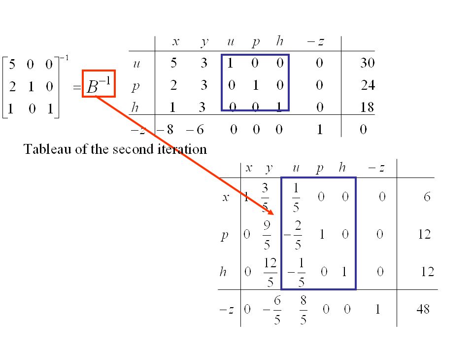
62. Tableau format of the simplex method
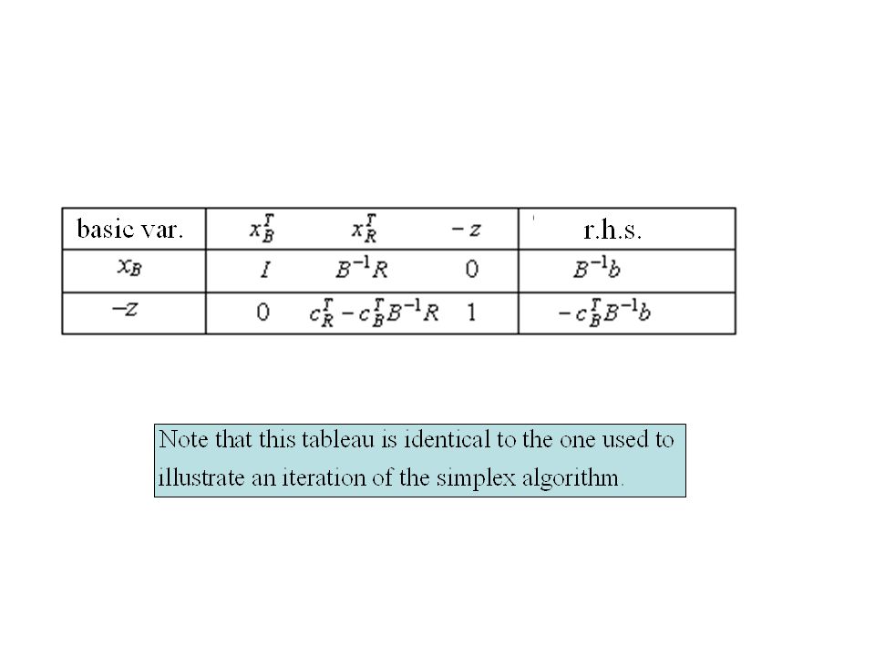
We now use the tableau format to complete the iterations of the simplex method.
We illustrate one iteration of the tableau format for solving the restaurant owner problem.

63. Recall the problem min z = –8x – 6y min z Sujet à Sujet à
5x + 3y + u = x + 3y + u =30
2x + 3y p = x + 3y p =24
1x + 3y h = x + 3y h = 18
x, y, u, p, h ≥ –8x –6y –z = 0
x, y, u, p, h ≥ 0

64. Equivalent tableau format for the system
min z = –8x – 6y min z
Subject to Subject to
5x + 3y + u = x + 3y + u =30
2x + 3y p = x + 3y p =24
1x + 3y h = x + 3y h = 18
x, y, u, p, h ≥ –8x –6y –z = 0
x, y, u, p, h ≥ 0
u = 30 – 5x – 3y
p = 24 – 2x – 3y
h = 18 – 1x – 3y
z = 0 –8x – 6y

65. u = 30 – 5x – 3y
p = 24 – 2x – 3y
h = 18 – 1x – 3y
z = 0 –8x – 6y
Step 1: Entering criterion
Determine the entering variable
by selecting the smallest element
in the last row of the tableau
min {–8, –6, 0, 0, 0} = –8.
x is then the entering variable

66. u = 30 – 5x – 3y
p = 24 – 2x – 3y
h = 18 – 1x – 3y
z = 0 –8x – 6y
Step 2: leaving criterion entering variable
To identify the leaving variable
determine the min of the ratio
right hand side terms divided by the
corresponding elements in the
column of the entering variable
that are positive:

67. u = 30 – 5x – 3y
p = 24 – 2x – 3y
h = 18 – 1x – 3y
z = 0 –8x – 6y
Step 2: leaving criterion entering variable
min {30/5, 24/2, 18} = 30/5 = 6
The corresponding variable u
becomes the leaving variable

68. u = 30 – 5x – 3y
p = 24 – 2x – 3y
h = 18 – 1x – 3y
z = 0 –8x – 6y
leaving variable entering variable
Step 3 : Pivot
Transform the system or
the tableau

69. 5x + 3y + u =30 leaving variable entering variable
RECALL: We use the equation including variable x and u to specify x in terms of u and y:
u = 30 – 5x – 3y => (5x = 30 – u – 3y) / 5
=> x = 6 – 1/5u – 3/5y
This is equivalent to
5x + 3y + u =30

70. (5x + 3y + u =30) / 5 leaving variable entering variable
RECALL: We use the equation including variable x and u to specify x in terms of u and y:
u = 30 – 5x – 3y => (5x = 30 – u – 3y) / 5
=> x = 6 – 1/5u – 3/5y
This is equivalent to
(5x + 3y + u =30) / 5

71. (5x + 3y + u =30) / 5 => x + 3/5y + 1/5u = 6
leaving variable
entering variable
RECALL: We use the equation including variable x and u to specify x in terms of u and y:
u = 30 – 5x – 3y => (5x = 30 – u – 3y) / 5
=> x = 6 – 1/5u – 3/5y
This is equivalent to
(5x + 3y + u =30) / 5 => x + 3/5y + 1/5u = 6

72. (5x + 3y + u =30) / 5 => x + 3/5y + 1/5u = 6
leaving variable
entering variable
This is equivalent to
(5x + 3y + u =30) / 5 => x + 3/5y + 1/5u = 6
In the tableau, this is equivalent to divide the row including the leaving variable by the coefficient of the entering variable in this row

73. (5x + 3y + u =30) / 5 => x + 3/5y + 1/5u = 6
Divide this row by 5
leaving variable
entering variable
This is equivalent to
(5x + 3y + u =30) / 5 => x + 3/5y + 1/5u = 6
In the tableau, this is equivalent to divide the row including the leaving variable by the coefficient of the entering variable in this row

74. Divide this row by 5
leaving variable
entering variable
We obtain the following tableau

75. Divide this row by
leaving variable
entering variable
We obtain the following tableau

76. Recall: Replace x in the other equations
x = 6 – 1/5u – 3/5y
p = 24 – 2x – 3y
=> p = 24 – 2(6 – 1/5u – 3/5y) – 3y
This is equivalent to : p = 24 – 2(6 – 1/5u – 3/5y) +2x – 2x – 3y
 2x + 3y + p – 2 (x + 3/5y +1/5u) = 24 – 2(6)

77. This is equivalent to : p = 24 – 2(6 – 1/5u – 3/5y) +2x – 2x – 3y
 2x + 3y + p – 2 (x +3/5y + 1/5u) = 24 – 2(6)
 x + 3y p = 24
– 2 (x +3/5y + 1/5u = 6)
0x + 9/5y –2/5u + p = 12
second row
minus
2(the first row)

78. Le tableau devient
second row
minus
2(the first row)

79. The tableau is modified as follows
second row
minus
2(the first row)

80. Doing this for the other rows of the tableau

81. Tableau format of the simplex method analysis of one iteration
Analyse one iteration of the tableau format of the simplex method
The system

82. can be written in the following tableau–

83. Step1: Select the entering variable
Referring to the last row of the tableau, let
If ≥ 0, then the current
solution is optimal, and
the algorithm stops
Entering variable
If < 0, then xs is the
entering variable –

84. Step 2: Select the leaving variableIf
the problem is not
bounded below,
and the alg. stops
Entering variable If
then the sol. remains feasible  –

85. Step 2: Select the leaving variable
Entering variable
Leaving variable –

86. Step 3: Pivot The pivot element is located at the intersection
of the column including the entering variable xs
and of the row including the leaving variable xr
Entering variable
Leaving variable –

87. Step 3: Pivot Devide row r by the pivot element to obtain a
new line r.
Variable d’entrée
Variable de sortie –

88. Step 3: Pivot Devide line r by the pivot element to obtain a
new line r.
Entering variable
Leaving variable –

89. Step 3: Pivot Multiply the new line r by ,
and substrack this from the line i. This induces that the coefficient of the entering variable xs to become equal to 0.
Entering variable
Leaving variable –

90. Step 3: Pivot Multiply the new line r by ,
and substrack this from the line i. This induces that the coefficient of the entering variable xs to become equal to 0.
Entering variable
Leaving variable –

91. Step 3: Pivot Multiply the new line r by ,
and substrack this from the line i. This induces that the coefficient of the entering variable xs to become equal to 0.
Entering variable
Leaving variable –

92. Step 3: Pivot Multiply the new line r by ,
and substrack this from the line i. This induces that the coefficient of the entering variable xs to become equal to 0.
Entering variable
Leaving variable –

93. New tableau for the next iteration–

94. Matrix notation

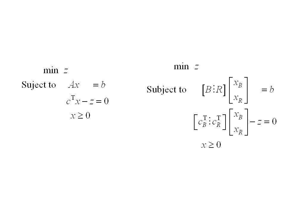
95. Matrix notation The linear programming problem in standard form min
Subject to

97. Matrix notation The linear programming problem in standard form min
Subject to

98. Matrix notation
min z
Subject to

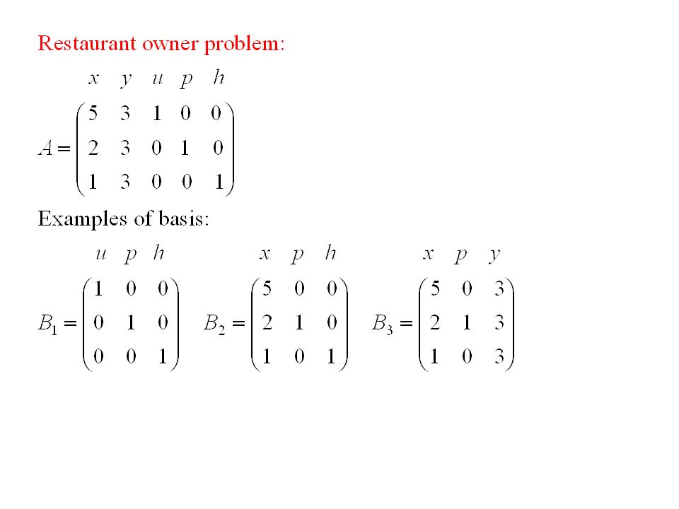
99. Matrix notation
Consider the matrix formulation of the linear programming problem
Assume that m ≤ n and that the matrix A is of full rank (i.e., rank(A) = m, or that the rows of A are linearly independent)
A sub matrix B of A is a basis of A if it is a mxm matrix and non singular (i.e, B-1 exists)

101. Matrix notation
A sub matrix B of A is a basis of A if it is a mxm matrix and non singular (i.e, B-1 exists)
To ease the presentation, assume that the basis B includes the first m columns of A, and then
Denote also
The original problem can be written as

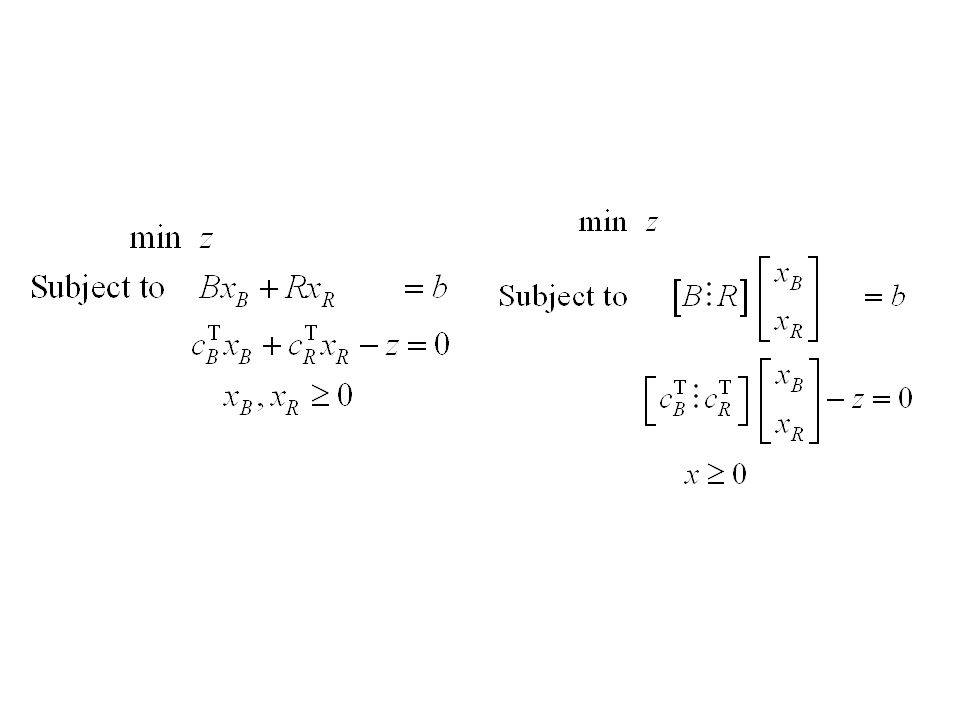
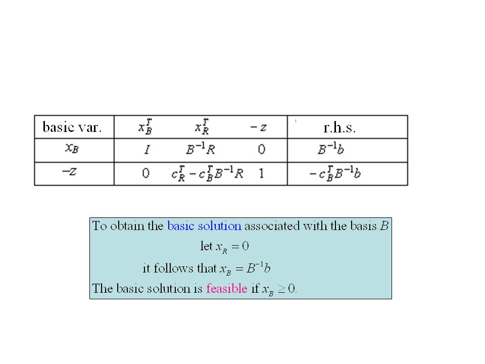
104. Specify xB in terms of xR using the constraints of the problem
Then

105. Replacing xB by its value in terms
of xR in the objective function
Note that the two problems are
equivalents since the second one is
obtained from the first one using
elementary operations based on a
non singular matrix B-1

106. Combining the coefficients of xR

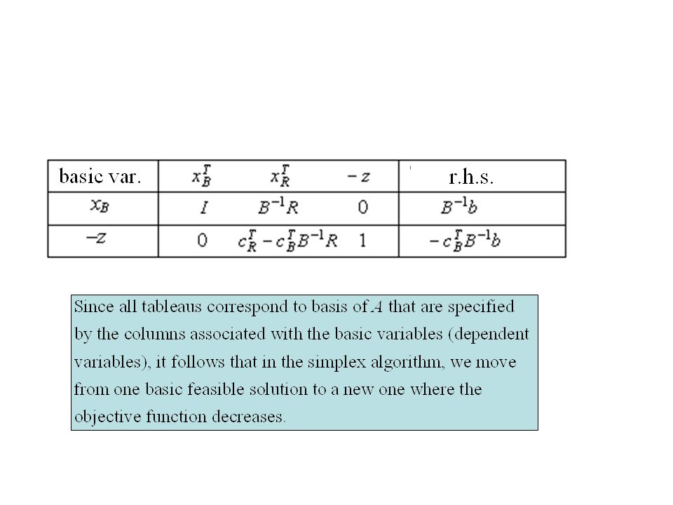
107. The problem can be specified in the following tableau

109. The variables xB (denoted as
the dependent variables)
associated with the columns
of the basis B, are now denoted
basic variables
The variables xR (denoted
independent variables)
are now denoted
non basic variables

112. -

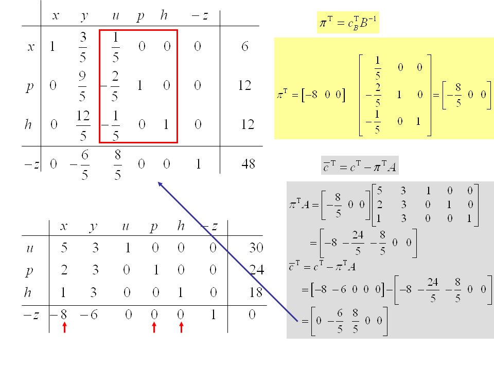
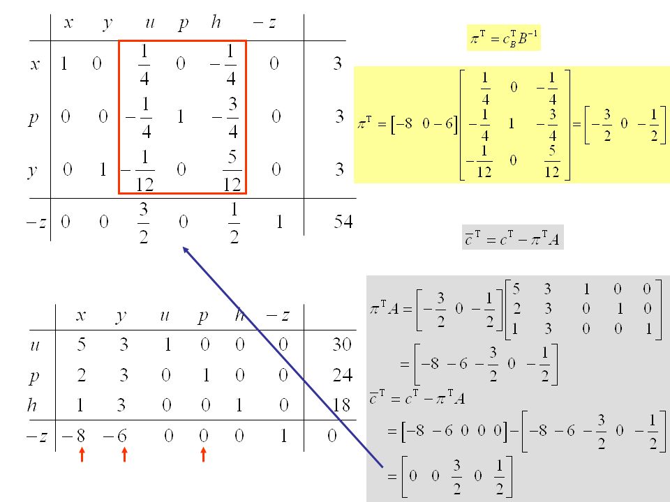
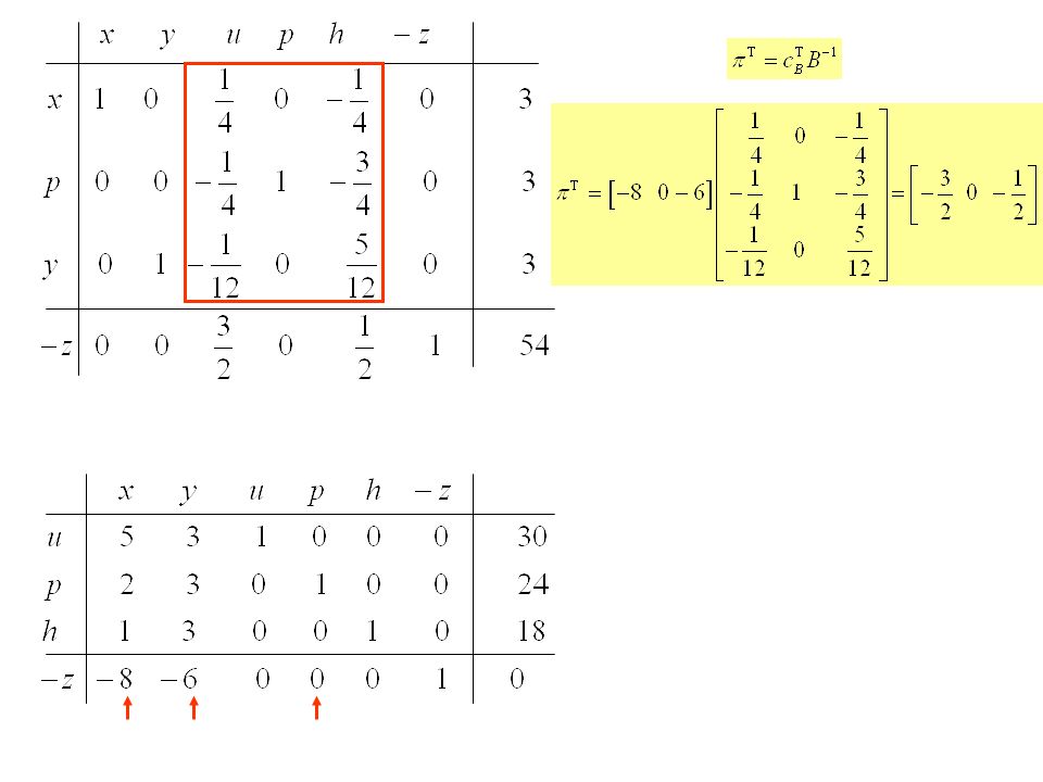
114. The simplex multipliers
Consider the last row of the simplex tableau corresponding to the
basis B associated to the relative costs of the variables:

115. The simplex multipliers
Consider the last row of the simplex tableau corresponding to the
basis B associated to the relative costs of the variables:

116. The simplex multipliers
Denote the vector specified by
Then or
where denotes the jth column of the contraint matrix A

119. The simplex multipliers

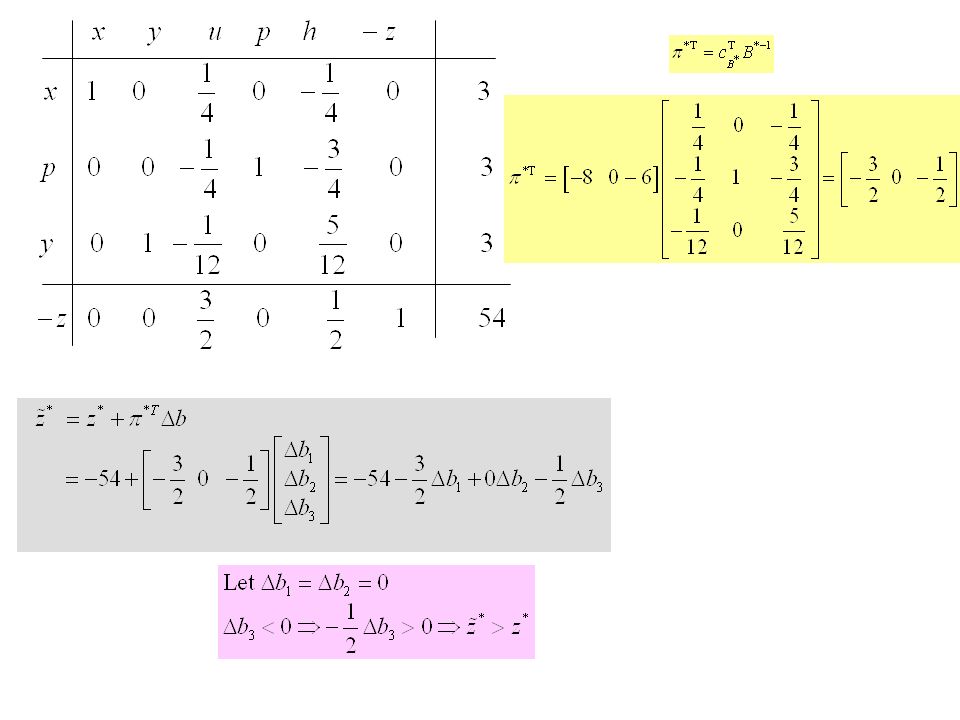
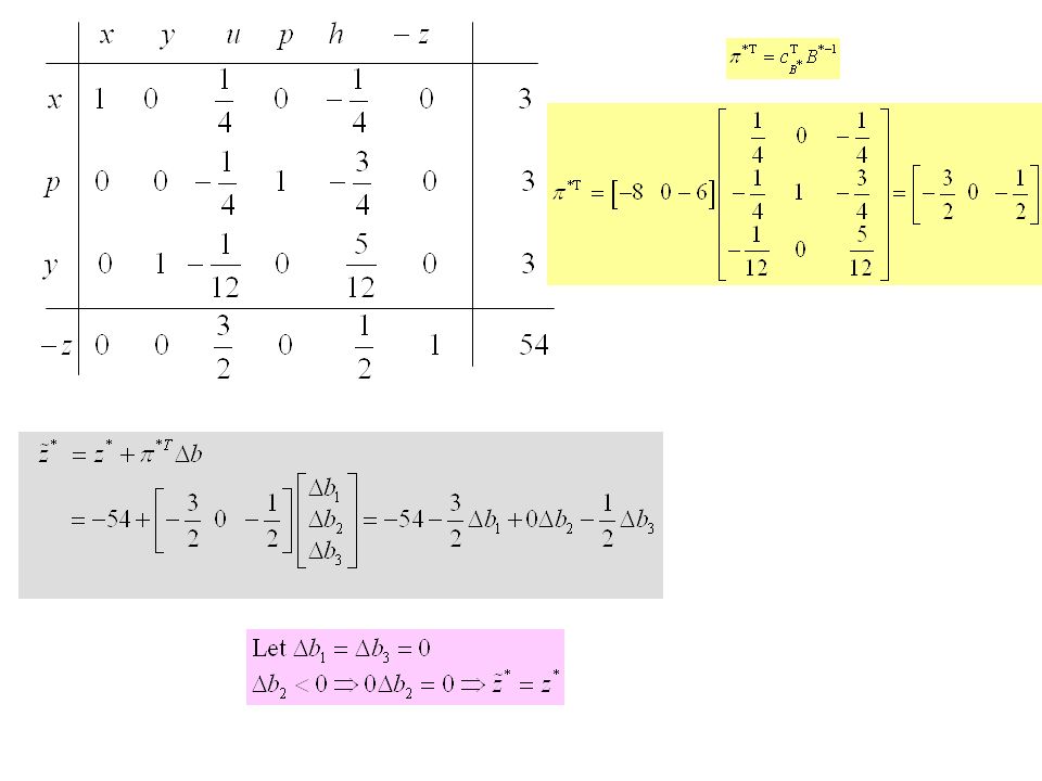
121. Sensitivity analysis of the optimal value when modifying the right hand side terms
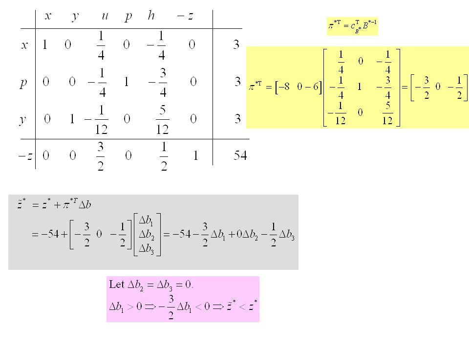
The simplex multipliers associated with an optimal basic solution allows to analyse the sensitivity of the optimal value when modfying the right hand terms.
Consider a problem and its version when modfying the right hand terms

122. Sensitivity analysis of the optimal value when modifying the right hand side terms
Let B* be an optimal basis, and the corresponding basic solution
having the optimal value

123. Sensitivity analysis of the optimal value when modifying the right hand side terms

124. Sensitivity analysis of the optimal value when modifying the right hand side terms

125. Sensitivity analysis of the optimal value when modifying the right hand side terms

126. Sensitivity analysis of the optimal value when modifying the right hand side terms

129. Feasible domain The feasible domain for the system 5x + 3y ≤ 30

130. Solving the problem graphicly
If b1 = 30 becomes b1+Δb1 with
Δb1<0
the size of the feasible domain is reduced
5x + 3y ≤ 30
2x + 3y ≤ 24
1x + 3y ≤ 18

132. Solving the problem graphicly
If b1 = 30 becomes b1+Δb1 with
Δb1>0
the size of the feasible domain is increased
5x + 3y ≤ 30
2x + 3y ≤ 24
1x + 3y ≤ 18

134. Solving the problem graphicly
If b3 = 18 becomes b3+Δb3 with
Δb3<0
the size of the feasible domain is reduced
5x + 3y ≤ 30
2x + 3y ≤ 24
1x + 3y ≤ 18

136. Solving the problem graphicly
If b2 = 24 becomes b2+Δb2 with
Δb2<0
the size of the feasible domain remains the same
5x + 3y ≤ 30
2x + 3y ≤ 24
1x + 3y ≤ 18

137. Optimality criterion
Proposition In the simplex algorithm, if at some iteration, all the relative costs , then the current solution is optimal
Proof: Without lost of generality, assume that the first m variables
x1, x2, …, xm are basic; i. e., -

138. Optimality criterion

139. Optimality criterion The objective function is as follows
Consider another feasible solution ≥ 0 with the value
But the hypothesis induces that

140. Optimality criterion The objective function is as follows
Consider another feasible solution ≥ 0 with the value
But the hypothesis induces that