1. future data scientists also need to be skilled in statistics, and to be able to tell stories with data, to make it understandable to a variety of people.

2. DNA microarray and array data analysis

4. What is DNA Microarray DNA microarray is a new technology to measure the level of the RNA gene products of a living cell. DNA microarray is a new technology to measure the level of the RNA gene products of a living cell. A microarray chip is a rectangular chip on which is imposed a grid of DNA spots. These spots form a two dimensional array. A microarray chip is a rectangular chip on which is imposed a grid of DNA spots. These spots form a two dimensional array. Each spot in the array contains millions of copies of some DNA strand, bonded to the chip. Each spot in the array contains millions of copies of some DNA strand, bonded to the chip. Chips are made tiny so that a small amount of RNA is needed from experimental cells. Chips are made tiny so that a small amount of RNA is needed from experimental cells.

5. DNA Microarray Many applications in both basic and clinical research Many applications in both basic and clinical research determining the role a gene plays in a pathway, disease, diagnostics and pharmacology, … determining the role a gene plays in a pathway, disease, diagnostics and pharmacology, … There are three main platforms for performing microarray analyses. There are three main platforms for performing microarray analyses. cDNA arrays (generic, multiple manufacturers) cDNA arrays (generic, multiple manufacturers) Oligonucleotide arrays (genechips) (Affymetrix) Oligonucleotide arrays (genechips) (Affymetrix) BeatArray (BeadChip) (Illumina) BeatArray (BeadChip) (Illumina) cDNA membranes (radioactive detection) cDNA membranes (radioactive detection)

6. cDNA Microarray Spot cloned cDNAs onto a glass/nylon microscope slide Spot cloned cDNAs onto a glass/nylon microscope slide usually PCR amplified segments of plasmids usually PCR amplified segments of plasmids Complementary hybridization Complementary hybridization -- CTAGCAGG actual gene -- GATCGTCC cDNA ( Reverse transcriptase) -- CUAGCAGG mRNA Label 2 mRNA samples with 2 different colors of fluorescent dye -- control vs. experimental Label 2 mRNA samples with 2 different colors of fluorescent dye -- control vs. experimental Mix two labeled mRNAs and hybridize to the chip Mix two labeled mRNAs and hybridize to the chip Make two scans - one for each color Make two scans - one for each color Combine the images to calculate ratios of amounts of each mRNA that bind to each spot Combine the images to calculate ratios of amounts of each mRNA that bind to each spot

7. CTRL TEST Spotted Microarray Process

8. cDNA Array Experiment Movie http://www.bio.davidson.edu/courses/genomic s/chip/chip.html http://www.bio.davidson.edu/courses/genomic s/chip/chip.html http://www.bio.davidson.edu/courses/genomic s/chip/chip.html http://www.bio.davidson.edu/courses/genomic s/chip/chip.html

9. Affymetrix Uses 25 base oligos synthesized in place on a chip (20 pairs of oligos for each gene) Uses 25 base oligos synthesized in place on a chip (20 pairs of oligos for each gene) cRNA labeled and scanned in a single “color” cRNA labeled and scanned in a single “color” one sample per chip one sample per chip Can have as many as 760,000 probes on a chip Can have as many as 760,000 probes on a chip Arrays get smaller every year (more genes) Arrays get smaller every year (more genes) Chips are expensive Chips are expensive Proprietary system: “black box” software, can only use their chips Proprietary system: “black box” software, can only use their chips

10. Affymetrix GeneChip ® Probe Arrays 24~50µm Each probe cell or feature contains millions of copies of a specific oligonucleotide probe Image of Hybridized Probe Array Single stranded, fluorescently labeled cRNA target Oligonucleotide probe * * * * * 1.28cm GeneChip Probe Array Hybridized Probe Cell *

11. GeneChip® Human Gene 1.0 ST Array

12. Affymetrix GeneChip ® Probe Array

13. Affymetrix Genome Arrays

14. Affymetrix GeneChip Probe: 25 bases long single stranded DNA oligos 25 bases long single stranded DNA oligos Probe Cell: Single square-shaped feature on an array containing one type of probe. Single square-shaped feature on an array containing one type of probe. Contains millions of probe molecules Contains millions of probe molecules Probe Pair: Perfect Match/Mismatch Perfect Match/Mismatch Probe Set

15. Perfect Match Mismatch 25 mer DNA oligo Array Design 3’ 5’ Twenty oligo probes are selected from the 3’ end of the gene For each probe selected, a partner containing a central mutation is also made Perfect Match Mismatch Probe Set Probe Pair PM MM Probe Cell 24  m For each gene a total of 20 probe pairs are arrayed on the chip

16. Probe Sub-types on chips Exemplars Specific transcripts 2. Expressed sequence tags (ESTs) 1. Known genes: Consensus 3. Spiked control transcripts Housekeeping genes

17. Total RNA (5-8  g) AAAAAAAAA cRNA preparation cRNA is now ready for hybridization to test chip cDNA Strand 1 synthesisTTTTTTTTTNNNNNNNNN AAAAAAAAA SS II reverse transcriptase T7RNA pol. promoter cDNA Strand 2 synthesis TTTTTTTTTNNNNNNNNN AAAAAAAAANNNNN E. coli DNA pol. I T7RNA pol. promoter NNNNNNNN IVT cRNA synthesis amplifies and labels transcripts with Biotin NNNNNNNNNNNNNAAAAAAAAAAAAAAN TTTTTT T T T T T UUUUUUUUUU ……….. UUUUUUUUUU ……….. UUUUUUUUUU ……….. UUUUUUUUUU ……….. UUUUUUUUUU ……….. …… ……. T 7 RNA pol. T T Fragmented cRNA

18. cDNA probes B B B B B B B B B B B B B B B B B BB B B cRNA labeled targets B B B B B B B B B B B BB B B Non- Specific Binding Specific Binding Post hybridiz -ation washes S FL S S

19. B B B S S S B B B S S S Streptavidin

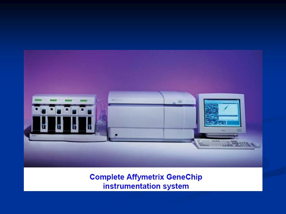
20. Chips are placed in the Fluidics station where they are washed, stained and washed again (2.5 hours) Chip is placed in a hybridization oven and incubated overnight Hybridization cocktail Affymetrix Array Chip Sample is added to a hybridization cocktail along with spiked control transcripts and is loaded onto an array chip Data is acquired by the computer as soon as the scan has been completed. After staining, the signal intensities are measured with a laser scanner (15 min)

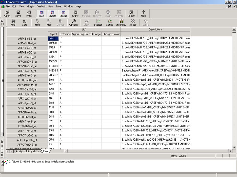
21. The chip image data file (or “.dat” file) is the first part of data acquisition and appears on the computer screen upon completion of the laser scan. Here, we zoom in to see an individual probe set that has been highlighted Probe set

22. The first image is “sample1.dat.” note the pixel to pixel variation within a probe cell A “*.cel.” file is automatically generated when the “*.dat” image first appears on the screen. Note that this derivative file has homogenous signal intensity within its probe cells

23. Affymetrix Algorithms 1.1 Adjusting MMs to purge negative values All MMs < PMs, No adjustment necessary Few MMs > PMs, change MMs based on weighted mean of other MMs Most MMs > PMs, change MMs to be slightly lesss than PM 1. Signal

24. Affymetrix Algorithms Signal Calculation. Calculate the signal PM 1000 5000 430 765 355 98 3005 413 20333 590 MM 900 2000 230 25 331 40 1200 203 6197 230 PM-MM 100 3000 200 740 24 58 1805 210 14136 360 Using Tukey’s biweight mean = 1780 Signal (expression level) = 1780 Having adjusted the MM values, we now calculate the signal The PM values.The PM-MM values are calculated.The MM values. Standard deviations 1 1 2 3 4 5 6 Weight factor The unweighted mean is vulnerable to outlier data. In order to protect against this, we dampen the effect of outliers by using the Tukey bi-weight mean. PM-MM values that are a number of standard deviations away from the mean are given low weights in accordance with the graph shown here. Individual PM-MM data are multiplied by the weight factor before calculation of the mean. The weighted mean is then called the “signal.” Unweighted mean = 2063

25. [CEL] Version=3 [HEADER] Cols=640 Rows=640 TotalX=640 TotalY=640 OffsetX=0 OffsetY=0 GridCornerUL=229 235 GridCornerUR=4496 269 GridCornerLR=4471 4534 GridCornerLL=204 4500 Axis-invertX=0 AxisInvertY=0 swapXY=0 DatHeader=[0..46132] CL2001031608AA:CLS=4733 RWS=4733 XIN=3 YIN=3 VE=17 2.0 03/16/01 13:32:23 HG_U95Av2.1sq 6 Algorithm=Percentile AlgorithmParameters=Percentile:75;CellMargin:2;OutlierHigh:1.500;OutlierLow:1.004 [INTENSITY] NumberCells=409600 CellHeader=XYMEANSTDVNPIXELS 0032596.725 106823.51007.720 2028456.925.cel file

28. Microarray Data Analysis Data processing and visualization Data processing and visualization Supervised learning Supervised learning Feature selection Feature selection Machine learning approaches Machine learning approaches Unsupervised learning Unsupervised learning Clustering and pattern detection Clustering and pattern detection Infer gene interactions in pathways and networks Infer gene interactions in pathways and networks Gene regulatory regions predictions based co-regulated genes Gene regulatory regions predictions based co-regulated genes Linkage between gene expression data and gene sequence/function databases Linkage between gene expression data and gene sequence/function databases …

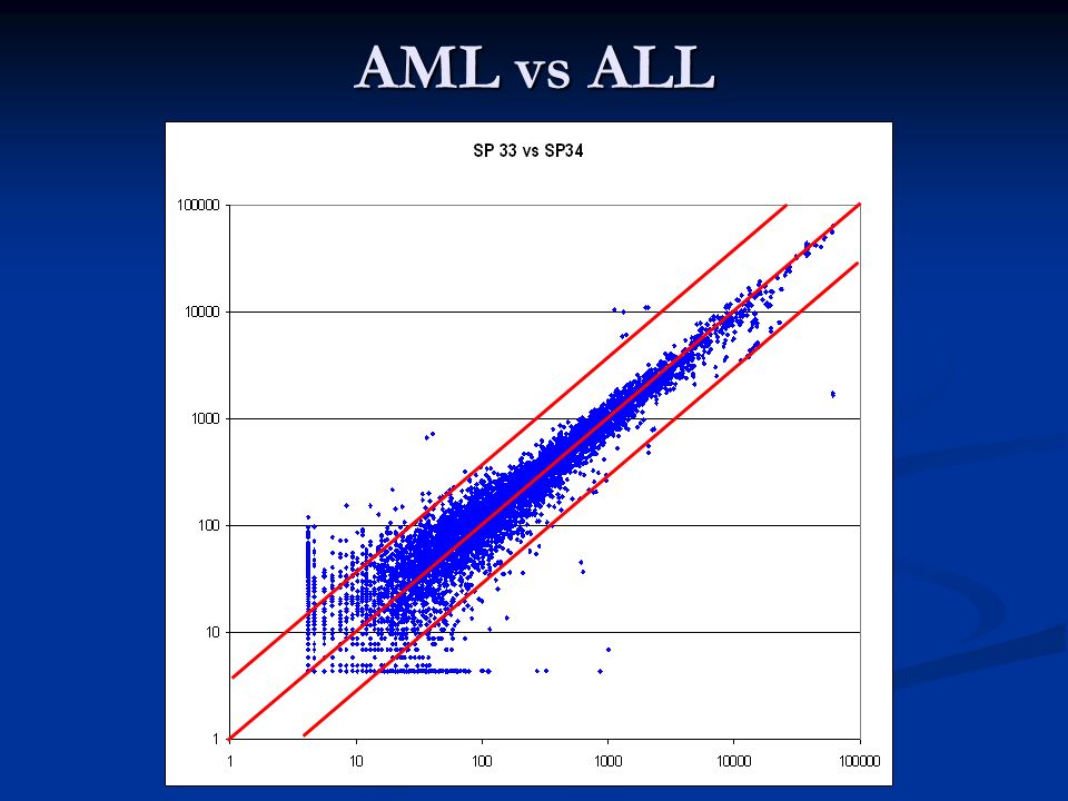
29. Microarrays: An Example Leukemia: Acute Lymphoblastic (ALL) vs Acute Myeloid (AML), Golub et al, Science, v.286, 1999 Leukemia: Acute Lymphoblastic (ALL) vs Acute Myeloid (AML), Golub et al, Science, v.286, 1999 72 examples (38 train, 34 test), about 7,000 probes 72 examples (38 train, 34 test), about 7,000 probes well-studied (CAMDA-2000), good test example well-studied (CAMDA-2000), good test example ALLAML Visually similar, but genetically very different

30. Normalization Need to scale the red sample so that the overall intensities for each chip are equivalent control Sample 1 Sample 2 What can we tell from the two plots ?

31. Normalization To insure the data are comparable, normalization attempts to correct the following variables: To insure the data are comparable, normalization attempts to correct the following variables: Number of cells in the sample Number of cells in the sample Total RNA isolation efficiency Total RNA isolation efficiency Signal measurement sensitivity Signal measurement sensitivity … Can use simple/complicated math Can use simple/complicated math Normalization by global scaling (bring each image to the same average brightness) Normalization by global scaling (bring each image to the same average brightness) Normalization by sectors Normalization by sectors Normalization to housekeeping genes Normalization to housekeeping genes … Active research area Active research area

32. AML vs ALL

34. Microarray Data Analysis Data processing and visualization Data processing and visualization Supervised learning Supervised learning Feature selection Feature selection Machine learning approaches Machine learning approaches Unsupervised learning Unsupervised learning Clustering and pattern detection Clustering and pattern detection Infer gene interactions in pathways and networks Infer gene interactions in pathways and networks Gene regulatory regions predictions based co-regulated genes Gene regulatory regions predictions based co-regulated genes Linkage between gene expression data and gene sequence/function databases Linkage between gene expression data and gene sequence/function databases …

35. Feature selection ProbeAML1AML2AML3ALL1ALL2ALL3 D21869_s_at170.755.043.75.5807.91283.5 D25233cds_at60531.0629.2441.795.3205.6 D25543_at2148.72303.01915.549.296.389.8 L03294_g_at241.8721.577.266.1107.3132.5 J03960_at774.53439.8614.355614.412.9 M81855_at10871283.71372.114694611.73211.8 L14936_at212.62848.5236.2260.52650.92192.2 L19998_at3673.2661.7629.4151193.9 L19998_g_at65.256.929.6434.0719.4565.2 AB017912_at1813.79520.62404.33853.16039.44245.7 AB017912_g_at385.42396.8363.7419.36191.95617.6 U86635_g_at83.3470.952.33272.53379.65174.6 …………………

36. ProbeAML1AML2AML3ALL1ALL2ALL3p-value D21869_s_at170.755.043.75.5807.91283.50.243 D25233cds_at60531.0629.2441.795.3205.60.487 D25543_at2148.72303.01915.549.296.389.80.0026 L03294_g_at241.8721.577.266.1107.3132.50.332 J03960_at774.53439.8614.355614.412.90.260 M81855_at10871283.71372.114694611.73211.80.178 L14936_at212.62848.5236.2260.52650.92192.20.626 L19998_at3673.2661.7629.4151193.90.941 L19998_g_at65.256.929.6434.0719.4565.20.022 AB017912_at1813.79520.62404.33853.16039.44245.70.963 AB017912_g_at385.42396.8363.7419.36191.95617.60.236 U86635_g_at83.3470.952.33272.53379.65174.60.022 ……………………   

37. Hypothesis Testing

38. Null hypothesis is a hypothesis set up to be nullified in order to support an alternative hypothesis. Null hypothesis is a hypothesis set up to be nullified in order to support an alternative hypothesis. Hypothesis testing is to test the viability of the null hypothesis for a set of experimental data Hypothesis testing is to test the viability of the null hypothesis for a set of experimental data Example: Example: Test whether the time to respond to a tone is affected by the consumption of alcohol Test whether the time to respond to a tone is affected by the consumption of alcohol Hypothesis : µ1 - µ2 = 0 Hypothesis : µ1 - µ2 = 0 µ1 is the mean time to respond after consuming alcohol µ1 is the mean time to respond after consuming alcohol µ2 is the mean time to respond otherwise µ2 is the mean time to respond otherwise ?

39. Z-test Theorem: If x i has a normal distribution with mean  and standard deviation  2, i=1,…,n, then U=  a i x i has a normal distribution with a mean E(U)=   a i and standard deviation D(U)=  2  a i 2. Theorem: If x i has a normal distribution with mean  and standard deviation  2, i=1,…,n, then U=  a i x i has a normal distribution with a mean E(U)=   a i and standard deviation D(U)=  2  a i 2.  x i /n ~ N( ,  2 /n).  x i /n ~ N( ,  2 /n). Z test : H: µ = µ 0 (µ 0 and  0 are known, assume  =  0 ) Z test : H: µ = µ 0 (µ 0 and  0 are known, assume  =  0 ) What would one conclude about the null hypothesis that a sample of N = 46 with a mean of 104 could reasonably have been drawn from a population with the parameters of µ = 100 and  = 8? Use What would one conclude about the null hypothesis that a sample of N = 46 with a mean of 104 could reasonably have been drawn from a population with the parameters of µ = 100 and  = 8? Use Note: z follows a normal distribution N(0, 1) Note: z follows a normal distribution N(0, 1)normal distribution N(0, 1)normal distribution N(0, 1) Reject the null hypothesis.

40. Z-test Theorem: If x i follows a normal distribution with mean  and standard deviation  2, i=1,…,n, then U=  a i x i has a normal distribution with a mean E(U)=   a i and standard deviation D(U)=  2  a i 2. Theorem: If x i follows a normal distribution with mean  and standard deviation  2, i=1,…,n, then U=  a i x i has a normal distribution with a mean E(U)=   a i and standard deviation D(U)=  2  a i 2.  x i /n ~ N( ,  2 /n).  x i /n ~ N( ,  2 /n). Z test : H: µ = µ 0 (µ 0 and  0 are known, assume  =  0 ) Z test : H: µ = µ 0 (µ 0 and  0 are known, assume  =  0 ) But, in practice  0 is often unknown.

41. T-test S x-y standard error of the difference Assuming  1 and  2 are different

42. William Sealey Gosset (1876-1937) William Sealey Gosset (1876-1937) (Guinness Brewing Company) T-test

43. P-value Does a particular gene have the same expression level in ALL and AML? ProbeAML1AML2AML3ALL1ALL2ALL3p-value D25543_at2148.72303.01915.549.296.389.80.0026 L03294_g_at241.8721.577.266.1107.3132.50.332 …………………… ALLAML

44. Data processing Feature selection Feature selection T-test T-test Based on the fold change Based on the fold change

45. Matlab ttest [H,P] = ttest2(X,Y) Determines whether the means from matrices X and Y are statistically different. H return a 0 or 1 indicating accept or reject null hypothesis (that the means are the same) P will return the significance level

46. Microarray Data Analysis Data processing and visualization Data processing and visualization Supervised learning Supervised learning Feature selection Feature selection Machine learning approaches Machine learning approaches Unsupervised learning Unsupervised learning Clustering and pattern detection Clustering and pattern detection Infer gene interactions in pathways and networks Infer gene interactions in pathways and networks Gene regulatory regions predictions based co-regulated genes Gene regulatory regions predictions based co-regulated genes Linkage between gene expression data and gene sequence/function databases Linkage between gene expression data and gene sequence/function databases …

47. Feature 2 Feature 1 L L L L L L L M M M M M M Nearest Neighbor Classification Nearest Neighbor Classification = AML = ALL = test sample M L Feature 2 Feature 1 L L L L L L L M M M M M M Feature 2 Feature 1 L L L L L L L M M M M M M = AML = ALL = test sample M L

48. Distance Issues Euclidean distance ■ Pearson distance g1g1 g2g2 g3g3 g4g4

49. Cross-validation http://en.wikipedia.org/wiki/Cross-validation_(statistics) http://en.wikipedia.org/wiki/Cross-validation_(statistics)

50. Microarray Data Analysis Data processing and visualization Data processing and visualization Supervised learning Supervised learning Feature selection Feature selection Machine learning approaches Machine learning approaches Unsupervised learning Unsupervised learning Clustering and pattern detection Clustering and pattern detection Gene regulatory regions predictions based co- regulated genes Gene regulatory regions predictions based co- regulated genes Linkage between gene expression data and gene sequence/function databases Linkage between gene expression data and gene sequence/function databases …

51. Genetic Algorithm for Feature Selection Sample Clear cell RCC, etc. Raw measurement data f1 f2 f3 f4 f5 Feature vector = pattern

52. Why Genetic Algorithm? Assuming 2,000 relevant genes, 20 important discriminator genes (features). Assuming 2,000 relevant genes, 20 important discriminator genes (features). Cost of an exhaustive search for the optimal set of features ? Cost of an exhaustive search for the optimal set of features ? C(n,k)=n!/k!(n-k)! C(2,000, 20) = 2000!/(20!1980!) ≥ (100)^20 = 10^40 If it takes one femtosecond (10 -15 second) to evaluate a set of features, it takes more than 3  10^17 years to find the optimal solution on the computer.

53. Evolutionary Methods Based on the mechanics of Darwinian evolution Based on the mechanics of Darwinian evolution The evolution of a solution is loosely based on biological evolution The evolution of a solution is loosely based on biological evolution Population of competing candidate solutions Population of competing candidate solutions Chromosomes (a set of features) Chromosomes (a set of features) Genetic operators (mutation, recombination, etc.) Genetic operators (mutation, recombination, etc.) generate new candidate solutions generate new candidate solutions Selection pressure directs the search Selection pressure directs the search those that do well survive (selection) to form the basis for the next set of solutions. those that do well survive (selection) to form the basis for the next set of solutions.

54. A Simple Evolutionary Algorithm Selection Genetic Operators Evaluation

55. Genetic Operators Crossover 10305070 20406080 Randomly Selected Crossover Point 1030 50702040 6080 Mutation 10306280 Randomly Selected Mutation Site l Recombination is intended to produce promising individuals. l Mutation maintains population diversity, preventing premature convergence.

56. Genetic Algorithm g2g1g6g3g21 g201g17g51g21g1 g12g7g15g12g10 g25g72g56g23g10 g20g7g5g2g100 Good enough Stop g20g7g6g3g21 g20g7g25g23g14 g12g7g15g22g10 g25g72g56g23g10 g2g1g5g2g100 Not good enough 5 2 1 4 3

57. GA Fitness At the core of any optimization approach is the function that measures the quality of a solution or optimization. At the core of any optimization approach is the function that measures the quality of a solution or optimization. Called: Called: Objective function Objective function Fitness function Fitness function Error function Error function measure measure etc. etc.

58. Encoding Most difficult, and important part of any GA Most difficult, and important part of any GA Encode so that illegal solutions are not possible Encode so that illegal solutions are not possible Encode to simplify the “evolutionary” processes, e.g. reduce the size of the search space Encode to simplify the “evolutionary” processes, e.g. reduce the size of the search space Most GA’s use a binary encoding of a solution, but other schemes are possible Most GA’s use a binary encoding of a solution, but other schemes are possible

59. Genetic Algorithm/K-Nearest Neighbor Algorithm Classifier (kNN) Feature Selection (GA) Microarray Database

60. Microarray Data Analysis Data processing and visualization Data processing and visualization Supervised learning Supervised learning Machine learning approaches Machine learning approaches Unsupervised learning Unsupervised learning Clustering and pattern detection Clustering and pattern detection Gene regulatory regions predictions based co- regulated genes Gene regulatory regions predictions based co- regulated genes Linkage between gene expression data and gene sequence/function databases Linkage between gene expression data and gene sequence/function databases …

61. Unsupervised learning Supervised methods Can only validate or reject hypotheses Can not lead to discovery of unexpected partitions Unsupervised learning No prior knowledge is used Explore structure of data on the basis of similarities

62. DEFINITION OF THE CLUSTERING PROBLEM

63. CLUSTER ANALYSIS YIELDS DENDROGRAM T (RESOLUTION)

64. BUT WHAT ABOUT THE OKAPI?

65. 5 24 13 Agglomerative Hierarchical Clustering 3 1 4 2 5 Distance between joined clusters Dendrogram at each step merge pair of nearest clusters initially : each point = cluster Need to define the distance between the new cluster and the other clusters. Single Linkage: distance between closest pair. Complete Linkage: distance between farthest pair. Average Linkage: average distance between all pairs or distance between cluster centers Need to define the distance between the new cluster and the other clusters. Single Linkage: distance between closest pair. Complete Linkage: distance between farthest pair. Average Linkage: average distance between all pairs or distance between cluster centers (UPGMA)

66. Hierarchical Clustering - Summary Results depend on distance update method Results depend on distance update method Greedy iterative process Greedy iterative process NOT robust against noise NOT robust against noise No inherent measure to identify stable clusters No inherent measure to identify stable clusters Average Linkage (UPGMA) – the most widely used clustering method in gene expression analysis

67. Cluster both genes and samples Sample should cluster together based on experimental design Sample should cluster together based on experimental design Often a way to catch labelling errors or heterogeneity in samples Often a way to catch labelling errors or heterogeneity in samples

68. nature 2002 breast cancer Heat map

69. Centroid methods – K-means Data points at X i, i= 1,...,N Centroids at Y ,  = 1,...,K Assign data point i to centroid  ; S i =  Cost E: E(S 1, S 2,...,S N ; Y 1,...Y K ) = Minimize E over S i, Y 

70. K-means “Guess” K=3

71. Start with random positions of centroids. K-means Iteration = 0

72. K-means Iteration = 1 Start with random positions of centroids. Assign each data point to closest centroid.

73. K-means Iteration = 2 Start with random positions of centroids. Assign each data point to closest centroid. Move centroids to center of assigned points

74. K-means Iteration = 3 Start with random positions of centroids. Assign each data point to closest centroid. Move centroids to center of assigned points Iterate till minimal cost

75. Fast algorithm: compute distances from data points to centroids Fast algorithm: compute distances from data points to centroids Result depends on initial centroids’ position Result depends on initial centroids’ position Must preset K Must preset K Fails for “non-spherical” distributions Fails for “non-spherical” distributions K-means - Summary

76. Issues in Cluster Analysis A lot of clustering algorithms A lot of clustering algorithms A lot of distance/similarity metrics A lot of distance/similarity metrics Which clustering algorithm runs faster and uses less memory? Which clustering algorithm runs faster and uses less memory? How many clusters after all? How many clusters after all? Are the clusters stable? Are the clusters stable? Are the clusters meaningful? Are the clusters meaningful?

77. Which Clustering Method Should I Use? What is the biological question? What is the biological question? Do I have a preconceived notion of how many clusters there should be? Do I have a preconceived notion of how many clusters there should be? How strict do I want to be? Spilt or Join? How strict do I want to be? Spilt or Join? Can a gene be in multiple clusters? Can a gene be in multiple clusters? Hard or soft boundaries between clusters Hard or soft boundaries between clusters