1. GRAPHICS OUTPUT PRIMITIVES CA 302 Computer Graphics and Visual Programming Aydın Öztürk aydin.ozturk@ege.edu.tr http://www.ube.ege.edu.tr/~ozturk

2. 1. Introduction Output Primitives: Point positions and line segments are the simplest geometric pirimitives. Other geometric pirimitives: Circles, conic sections, spline curves and surfaces

3. 2. Coordinate Reference Frame To describe a picture first we define a world coordinate reference frame (2D or 3D). Next, we describe the positions of the objects in world coordinates. These coordinate positions along with other information such as color are stored. Objects are then displayed by passing the scene information to the viewing routines.

4. 2. Coordinate Reference Frame 0 1 2 3 4 5 Locations on a video monitor are referenced in integer screen coordinates which correspond to pixel positions in the frame buffer. 5 14 3 1 0 2 1

5. 2. Coordinate Reference Frame Once pixel positions have been identified for an object, the appropriate color values must be stored in the frame buffer. For this purpose we assume that we have the low-level Procedures setPixel (x,y) getPixel (x,y, color)

6. 3. Specifying a 2D World-Coordinate System in OpenGL The OpenGl commands for setting up a 2D Cartesianreference frame are glMatrixMode (GL_PROJECTION); glLoadIdentity (); gluOrtho2D (xmin, xmax, ymin, ymax) We add an identity matrix before the projection matrix to ensure that the coordinate values were not accumulated with any previously computed values.

7. 4. OpenGL Point Functions We use the following OpenGl function to state the coordinate values of a single point glBegin (GL_POINTS); glVertex * ( ); glEnd; where ( * ) indicates that suffix codes are required for this function.

8. 4. OpenGL Point Functions (cont.) Alternatively we can specify the coordinate values as int point1 [ ]={50, 100}; int point2 [ ]={75, 150}; int point3 [ ]={100, 200}; and call the OpenGL function to plot these points as(v is for vector) glBegin (GL_POINTS); glVertex2iv (point1); glVertex2iv (point2); glVertex2iv (point3); glEnd;

9. 4. OpenGL Line Functions (cont.) glBegin (GL_LINES); glVertex2iv (point1); glVertex2iv (point2); glVertex2iv (point3); glEnd; p3p3 p1p1 p4p4 GL_LINES p5p5 p1p1 p4p4 p2p2 p3p3 p5p5 p1p1 p4p4 p2p2 p3p3 p2p2 GL_LINE_STRIPGL_LINE_LOOP

10. 5. Line Drawing Algorithms The line equation For a given interval the corrresponding y -interval can be computed as x0x0 x end y0y0 y end

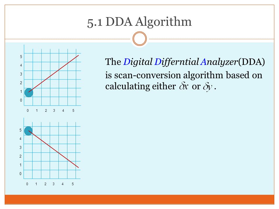
11. 5.1 DDA Algorithm 0 1 2 3 4 5 The Digital Differntial Analyzer(DDA) is scan-conversion algorithm based on calculating either or. 5 4 3 0 2 1 0 1 2 3 4 5 5 4 3 0 2 1

12. 5.1 DDA Algorithm(cont.) xkxk For m<1 : For m>1 : ykyk

13. 5.1 DDA Algorithm(cont.) Since m is a real number, each calculated x or y values must be rounded to the integer. DDA is a fast algorithm. Accumulation of round-off error in successive additions of the increments can couse a serios problem.

14. 5.2 Bresenham’s Line Algorithm Bresenham’s Line Algorithm uses only inremental integer calculations. When sampling at unit x intervals, we decide about which of the two pixel positions is closer to the true line path at each step. x k x k+1 x k+2 x k+3 x k+4 x k+5 y k+3 y k+2 y k+1 ykyk y=mx+b

15. 5.2 Bresenham’s Line Algorithm(cont.) x k +1 y k +1 y ykyk d lower d upper

16. 5.2 Bresenham’s Line Algorithm(cont.) To determine which of the two pixels is closest to the line path, a test is made based on the following quantity: or equivalently where

17. 5.2 Bresenham’s Line Algorithm(cont.) The sign of p k is the same as the sign since c is a constant and eliminated in the recursive calculations. We plot the lower pixel if p < 0 otherwise we plot the upper pixel.

18. 5.2 Bresenham’s Line Algorithm(cont.) We can calculate p k recursively as follows:

19. 5.2 Bresenham’s Line Algorithm(cont.) Finding the inital value p 0

20. 5.2 Bresenham’s Line Algorithm(cont.) The algorithm 1. Input the line end poins and store (x 0, y 0 ). 2.Set the color for frame-buffer position (x 0, y 0 ); (i.e. Plot the firs point). 3. Calculate the constants and find. 4. At each x k starting at k=0, perform the following test: If, then the next point to plot is Otherwise the next point to plot is 5.Perform step 4 times.

21. 5.3 Line Drawing Using Parametric Line Equations A parametric line equation in 2D that goes through points P 0 = (x 0, y 0 ) and P 1 = (x 1, y 1 ) can be written as

22. 5.3 Line Drawing Using Parametric Line Equations A nice property of this algorithm is that it works whether or not x 1 >x 2. An incremental pseudo code for this algorithm is

23. 6. Circle-Generating Algorithms xcxc ycyc (x,y) r θ A point (x,y ) on a circle can be expressed by the equation For a given x, the corresponding y-value can be calculated as

24. 6.1. Midpoint Circle Algorithm To apply the mid-point method we define Assuming that the point (x k, y k ) was plotted, we determine whether the next pixel at position (x k+1, y k ) or at position (x k+1, y k ). l Midpoint y k-1 ykyk x k+1 xkxk x k+2

25. 6.1. Midpoint Circle Algorithm The decision function is defined as A recursive expression for the next position at position x k+1 +1= x k +2 is

26. 6.1. Midpoint Circle Algorithm or where y k+1 is either y k or y k-1 depending on the sign of p k.

27. 6.1. Midpoint Circle Algorithm The initial decision parameter is obtained as follows: If r is defined as an integer, p 0 can be raunded to p 0 =1-r

28. 6.1. Midpoint Circle Algorithm The algorithm: 1. Input radius r and circle center ( x c y c ) then set the coordinates for the first point as (( x 0 y 0 )=( 0, r). 2. Calculate the initial value of the decision parameter as 3.At each x k position, starting at k= 0, perform the following test: if p k < 0, the next point is at ( x k+1, y k ) and otherwise the next point is at ( x k +1, y k -1 ) and

29. 6.1. Midpoint Circle Algorithm The algorithm: 4. Determine symmetry points in the other oktants. 5. Move each point onto the circle centered at (x c, y c ). 6. Repeat steps 3 until x≥y.

30. 7. Fill-Area Primitives Another useful costruct, besides points, straight-line segments, and curves for describing components of a picture is an area that is filled with some solid color or pattern. A picture component of this type is referred to as fill area. Mostly, fill areas are used to describe solid objects.

31. 7.1. Polygon Fill-Areas Polygon Classification: Convex polygon: All interior angles are ≤180 0. Concave polygon: A polygon that is not convex

32. 7.1. Polygon Fill-Areas Identifying Concave Polygons A Concave poligon has at least one interior angle greater than 180 0. Extension of some edges of a concave polygon intersect other edges. Some pair of interior points in a concave polygon produces a line segment that intesects the polygon boundary

33. Polygon Fill Convex Concave <180 o lE1lE1 lE2lE2 lE3lE3 lE4lE4 lE5lE5 lE6lE6 >180 o

34. 7.1. Polygon Fill-Areas Splitting Concave Polygons Once we have identified a concave poligon we can split it into a set of convex polygons. This can be accomplished using edge vectors and edge cross products. We first need to form the edge vectors E k = V k+1 -V k. Next we calculate cross products of successive edge vectors in order around the poligon perimeter. If the z-component of some cross products is positive while other cross products have a negative z-component, the polygon is concave.

35. 7.1. Polygon Fill-Areas ( E 1 × E 2 ) z >0 ( E 2 × E 3 ) z >0 ( E 3 × E 4 ) z <0 ( E 4 × E 5 ) z >0 ( E 5 × E 6 ) z >0 E1E1 E2E2 E3E3 E4E4 E5E5 E6E6 Splitting A Concave Poligon

36. 7.1. Polygon Fill-Areas Example E1E1 E2E2 E3E3 E4E4 E5E5 E6E6

37. 7.1. Polygon Fill-Areas Splitting of a Polygon into Triangles OpenGL guarentees correct rendering of polygons only if they are convex. A triangle is a convex polygon. But a polygon which has >3 vertices can be concave. So, we must tesselate a given polygon into triangles.The GLU library has a tesselator.

38. 7.1. Polygon Fill-Areas: Inside-Outside Testing We want fill inside of a polygon with constant color Flat and Convex polygons are guarenteed to be rendered correctly by OpenGL. For non-flat polygons:  We can work with their projections.  Or we can use first three vertices to determine a flat plane to use for the interrior. For non-simple flat polygons, we must decide how to determine whether a given point is inside or outside of the polygon.

39. 7.1. Polygon Fill-Areas: Inside-Outside Testing

40. Odd-even rule (easy implementation) crossing, odd parity rule, even-odd rule Crossed odd edges : inside point Crossed even edges : outside point Non-zero winding rule Clocwise edges : +1 Counterclocwise edges : –1 Don’t fill while total 0 7.1. Polygon Fill-Areas: Inside-Outside Testing

41. 7.2. Polygon Tables VERTEX TABLE V1: x1 y1 z1 V2: x2 y2 z2 V3: x3 y3 z3 V4: x4 y4 z4 V5: x5 y5 z5 EDGE TABLE E1 : V 1, V 2 E2 : V 2, V 3 E3 : V 3, V 1 E4 : V 3, V 4 E5 : V 4, V 5 E6 : V 5, V 1 POLYGON-SURFACE TABLE S1 : E1, E 2, E3 S2 : E 3, E4, E5, E6 E1 S1 S2 V2 V5 V1 V3 V4 E2 E4 E5 E6 E3

42. 7.2. Polygon Tables E1 S1 S2 V2 V5 V3 V4 E2 E4 E5 E6 E3 Edge Table for the surfaces EDGE TABLE E1 : V 1, V 2, S1 E2 : V 2, V 3, S1 E3 : V 3, V 1, S1, S2 E4 : V 3, V 4, S2 E5 : V 4, V 5, S2 E6 : V 5, V 1, S2

43. 7.3. Planes (x, y, z)

44. 7.3.1 Plane Equations (x, y, z)

45. 7.3.2 Front and Back Polygon faces For any point (x, y, z) on a plane we have For any point (x, y, z) behind the plane we have For any point (x, y, z) is infront of the plane we have l

46. 7.3.2 Front and Back Polygon faces Orientation of a polygon surface can be described with the normal vector for the plane. The cartesian coordinates of the normal is (A, B, C). l x y z V2 V1 V3 N

47. 7.3.2 Front and Back Polygon faces The elements of normal vector can also be obtained using a vector cross product. In a rigthanded Cartesian system if we select the vertex positions V 1, V 2, V 3 taken in the counter clockwise order when viewing from outside the object toward the inside we have l x y z V2 V1 V3 N

48. 7.3.2 Front and Back Polygon faces For any point P on the plane, the plane equation can be written as l

49. 7.3.2 Front and Back Polygon faces Example: Find the plane equation for the points V 1 =(1, 2, 3), V 2 =( 4, 3, 8), V 3 =(8, 13, 16) First, de define the vectors on in the plane as P 1 = V 2 - V 1 = ( 3, 1, 5) P 2 = V 3 - V 1 = ( 7, 11, 13) and find the normal vector as N= P 1 ×P 2 = (-29, -4, 19) Next, using one of the points in the plane (e.g. V 1 ), NV 1 = -D = 20 we obtain the plain equatin as -29X -4Y+19Z-20=0 l

50. 7.4 OpenGL Polygon Fill-Area Functions By default, a polygon interior is displayed in a solid color. In OPENGL, a fill area must be specified as a convex polygon. A polygon vertex list must contain at least three vertices. l glBegin (GL_POLYGON); glvertex2iv (p1); glvertex2iv (p2); glvertex2iv (p3); glvertex2iv (p4); glvertex2iv (p5); glvertex2iv (p6); glEnd( ) p1 p2p3 p4 p5 p6

51. 7.4 OpenGL Polygon Fill-Area Functions Reordering the vertex list and change the pirimitive constant in the previous code, we obtain different shapes. For example l glBegin (GL_TRIANGLES); glvertex2iv (p1); glvertex2iv (p2); glvertex2iv (p6); glvertex2iv (p3); glvertex2iv (p4); glvertex2iv (p5); glEnd ( ); p1 p2p3 p4 p5 p6

52. 7.4 OpenGL Polygon Fill-Area Functions Reordering the vertices and changing the primitive constant to GL_TRIANGLE_STRIP results the following shape l glBegin (GL_TRIANGLE_STRIP); glvertex2iv (p1); glvertex2iv (p2); glvertex2iv (p6); glvertex2iv (p3); glvertex2iv (p5); glvertex2iv (p4); glEnd ( ); p1 p2p3 p4 p5 p6

53. 7.4 OpenGL Polygon Fill-Area Functions l glBegin(GL_TRIANGLE_FAN); glvertex2iv (p1); glvertex2iv (p2); glvertex2iv (p3); glvertex2iv (p4); glvertex2iv (p5); glvertex2iv (p6) glEnd ( ); p1 p2p3 p4 p5 p6

54. 7.4 OpenGL Polygon Fill-Area Functions OpenGL providesfor the specifications of two types of four sided polygons(quadrileterals): GL_QUADS and GL_QUAD_STRIP) l glBegin(GL_QUADS); glvertex2iv (p1); glvertex2iv (p2); glvertex2iv (p3); glvertex2iv (p4); glvertex2iv (p5); glvertex2iv (p6); glvertex2iv (p7); glvertex2iv (p8); glEnd ( ); p1 p2 p3 p4 p5 p6 p7 p8

55. 7.4 OpenGL Polygon Fill-Area Functions l glBegin(GL_QUAD_STRIP); glvertex2iv (p1); glvertex2iv (p2); glvertex2iv (p4); glvertex2iv (p3); glvertex2iv (p5); glvertex2iv (p6); glvertex2iv (p8); glvertex2iv (p7); glEnd ( ); p1 p2 p3 p4 p5 p6 p7 p8

56. 7.5 OpenGL Vertex Arrays There are a number of ways for defining the vertex coordinates. Example : Drawing a cube. l typedef Glint vertex3 [3]; Vertex3 pt [8] = {{0, 0,0}, {0, 1, 0}, {1, 0, 0}, {1, 1, 0}, {0, 0,1}, {0, 1, 1}, {1, 0, 1}, {1, 1, 1}} 1 2 3 4 5 6 7 0 y x z

57. 7.5 OpenGL Vertex Arrays Code for drawing a cube: l void quad (GLint n1, GLint n2, GLint n3, GLint n4) { glBegin [GL_quads); glVertex3iv (pt [n1]); glVertex3iv (pt [n2]); glVertex3iv (pt [n3]); glVertex3iv (pt [n4]); glEnd ( ); } void cube ( ) { quad(6, 2, 3, 7); quad(5, 1, 0, 4); quad(7, 3, 1, 5); quad(4, 0, 2, 6); quad(2, 0, 1, 3); quad(7, 5, 4, 6); }

58. 7.6 OpenGL Pixel-Array Functions l A pattern defined as an array of color values is applied to a block of frame-bufferpi xel positions with the function glDrawPixels (width, height, dataFormat, dataType, pixMap);  Parameters width and height give the column and row dimensions respectively of the array pixMap.  dataFormat is assigned an OpenGL constant that indicates how thw values are specified for the array(for example: GL_BLUE specify a single blue color for all pixels, GL_BGR specify three color components in the order blue,green, red).  dataType : GL_BYTE, GL_INT, or GL_FLOAT. Example: Display a pixmap defined in a 128×128 array of RGB colors: glDrawPixels (128, 128, GL_RGB, GL_UNSIGNED_BYTE, colorshape);

59. 7.6 OpenGL Pixel-Array Functions l A single color buffer is selected for storing a pixmap with the command glDrawBuffer (buffer); The paprameter buffer can be assigned to one of the following constants: GL_FRONT_LEFT GL_FRONT_RIGHT GL_BACK_LEFT GL_BACK_RIGHT GL_FRONT (selects both front buffers)

60. 7.7 OpenGL Raster Operations l In addition to storing an array of pixel values in a buffer we can retrieve a block of values from a buffer or copy the block into another buffer area. Raster operation is used to describe to any function that processes a pixel array in some way.  A raster operation that moves an array of pixel values from one place to another is referred to as block transfer of pixel values.

61. 7.7 OpenGL Raster Operations l To select a rectangular block of pixel values in a designated set of buffers: glReadPixels (xmin, ymin, width, height, dataFormat, dataType, array) To copy a rectangular block of pixel data from one location to another : glCopyPixels (xmin, ymin, width, height, pixel values)