1. Discrete Distributions
CIVL 7012/8012
Discrete Distributions

2. Definitions
A random variable is a “function” that associates a unique numerical value with every outcome of an experiment. A probability distribution is a “function” that defines the probability of occurrence of every possible value that a random variable can take on.

3. Probability Distributions
There are two general types of probability distributions:
Discrete
Continuous
A discrete random variable can only take on discrete (i.e., specific) values.
A continuous random variable takes on continuous values (i.e., real values).

4. Properties of Discrete Distributions
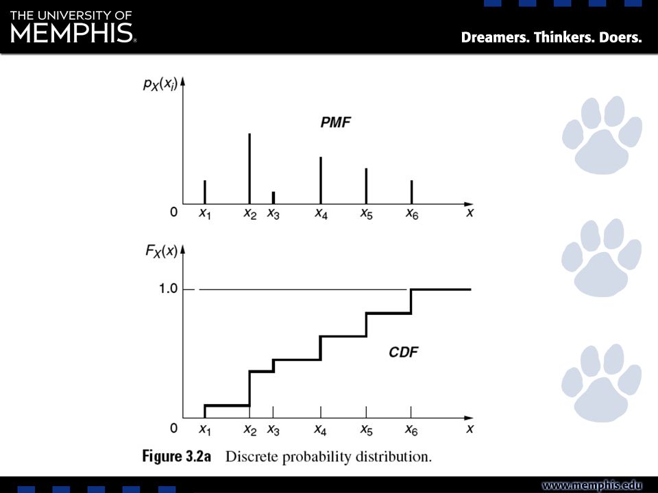
The probability mass function (PMF) gives the probability that the random variable X will take on a value of x when the experiment is performed:
By definition, p(x) is always a number between zero and one:
and, since every trial must have exactly one outcome,

6. Properties of Discrete Distributions
The cumulative distribution function (CDF) gives the probability that the
random variable X will take on a value less than or equal to x
when the experiment is performed:
The expected value of a random variable is the probability-weighted
average of the possible outcomes:

7. Properties of Discrete Distributions
The variance of a probability distribution is a measure of the
amount of variability in the distribution of the random variable, X,
about its expected value.
Mathematically, the variance is just the probability-weighted
average of the squared deviations:
We can also calculate the variance as:

8. Bernoulli Trials
To be considered a Bernoulli trial, an experiment must meet
three criteria:
There must be only 2 possible outcomes.
Each outcome must have an invariant probability of occurring.
The probability of success is usually denoted by p, and the probability
of failure is denoted by q = 1 – p.
3. The outcome of each trial is completely independent of the outcome
of any other trials.

9. Discrete Distributions
Binomial Distribution – Probability of exactly X successes in n trials.
Negative Binomial – Probability that it will take exactly n trials to produce exactly X successes.
Geometric Distribution – Probability that it will take exactly n trials to produce exactly one success. (Special case of the negative binomial).
Hypergeometric Distribution – Probability of exactly X successes in a sample of size n drawn without replacement.
Poisson Distribution – Probability of exactly X successes in a “unit” or continuous interval.

10. Binomial Distribution
Gives the probability of exactly x successes in n trials
A. Requirements
There must be x successes and (n – x) failures in the n trials, but the order
in which the successes and failures occur is immaterial.
B. Mathematical Relationships
1. General Equation:
where
n = the number of trials
x = the number of successes
p = the probability of a success for any given trial
q = 1 – p = the probability of a failure for any given trial
= the Binomial Coefficient

11. Binomial Distribution
2. Expectation – the expected (mean) number of successes in n trials
3. Variance – the expected sum of the squared deviations from the mean

12. Binomial Distribution Shapes
Figure 3-8 Binomial Distributions for selected values of n and p. Distribution (a) is symmetrical, while distributions (b) are skewed. The skew is right if p is small.
© John Wiley & Sons, Inc. Applied Statistics and Probability for Engineers, by Montgomery and Runger

13. Examples:
The probability that a certain kind of component will survive a given shock test is ¾. Find the probability that exactly two of the next four components tested survive.
The drainage system of a city has been designed for a rainfall intensity that will be exceeded on an average once in 50 years. What is the probability that the city will be flooded at most 2 out of 10 years?

14. Negative Binomial Distribution
Gives the probability that it will take exactly n trials to produce exactly x successes. A. Requirements The last (nth) trial must be a success, otherwise the xth success actually occurred on an earlier trial. This means that we must have (x – 1) successes in the first (n – 1) trials plus success on the nth trial. B. Mathematical Relationships 1. General Equation:
Our textbook:

15. Negative Binomial Distribution
2. Expectation – the expected number of trials to produce x successes 3. Variance – the expected sum of the squared deviations from the mean.

16. Negative Binomial Graphs
Figure Negative binomial distributions for 3 different parameter combinations.
© John Wiley & Sons, Inc. Applied Statistics and Probability for Engineers, by Montgomery and Runger

17. Example
Cotton linters used in the production of rocket propellant are subjected to a nitration process that enables the cotton fibers to go into solution. The process is 90% effective in that the material produced can be shaped as desired in a later processing stage with probability What is the probability that exactly 20 lots will be produced in order to obtain the third defective lot?

18. Geometric Distribution
Gives the probability that it will take exactly n trials to produce the first success.
A. Requirements
The first success must occur on the nth trial, so we must have (n – 1) failures
in the first (n – 1) trials plus success on the nth trial.
B. Mathematical Relationships
1. General Equation
Substituting (x = 1) into the Negative Binomial equation:
or:

19. Geometric Distribution
2. Expectation – the expected number of trials to produce x successes 3. Variance – the expected sum of the squared deviations from the mean.

20. Example
In a certain manufacturing process, it is known that, on the average, 1 in every 100 items is defective. What is the probability that the fifth item inspected is the first defective item found?

21. Lack of Memory Property
Let X1 denote the number of trials to the 1st success.
Let X2 denote the number of trials to the 2nd success, since the 1st success.
Let X3 denote the number of trials to the 3rd success, since the 2nd success.
Let the Xi be geometric random variables – independent, so without memory.
Then X = X1 + X2 + X3
Therefore, X is a negative binomial random variable, a sum of three geometric rv’s.
© John Wiley & Sons, Inc. Applied Statistics and Probability for Engineers, by Montgomery and Runger

22. Recap Binomial distribution: Fixed number of trials (n).
Random number of successes (x).
Negative binomial distribution:
Random number of trials (x).
Fixed number of successes (r).
Because of the reversed roles, a negative binomial can be considered the opposite or negative of the binomial.
© John Wiley & Sons, Inc. Applied Statistics and Probability for Engineers, by Montgomery and Runger

23. Hypergeometric Distribution
This distribution is fundamentally different from binomial distributions. The trials for hypergeometric are NOT INDEPENDENT. (Items are selected without replacement). Useful for acceptance sampling, electronic testing, quality assurance.
Given a set of N items, K of which have a trait of interest (“successes”), we wish to select a sample of n items without replacement from the set N. The variable x represents the number of successes in the n items.

24. Hypergeometric Distribution
A set of N objects contains:
K objects classified as success
N - K objects classified as failures
A sample of size n objects is selected without replacement from the
N objects, where:
K ≤ N and n ≤ N
© John Wiley & Sons, Inc. Applied Statistics and Probability for Engineers, by Montgomery and Runger

25. Hypergeometric Distribution
If X is a hypergeometric random variable with parameters N, K, and n, then
Sampling with replacement is equivalent to sampling from an infinite set because the proportion of success remains constant for every trial in the experiment. Thus, the only way the variance of the hypergeometric differs from the binomial is due to the finite population correction factor.
σ2 approaches the binomial variance as n /N becomes small.
© John Wiley & Sons, Inc. Applied Statistics and Probability for Engineers, by Montgomery and Runger

26. Hypergeometric Graphs
Figure Hypergeometric distributions for 3 parameter sets of N, K, and n. 26
© John Wiley & Sons, Inc. Applied Statistics and Probability for Engineers, by Montgomery and Runger

27. Hypergeometric & Binomial Graphs
Figure Comparison of hypergeometric and binomial distributions. 27
© John Wiley & Sons, Inc. Applied Statistics and Probability for Engineers, by Montgomery and Runger

28. Example
A particular part that is used as an injection device is sold in lots of 10. The producer deems the lot acceptable if no more than one defective part is in the lot. Some lots are sampled, and the sampling plan involves random sampling and testing 3 of the parts out of 10. If none of the three parts are defective, the lot is accepted. Comment on the utility of this plan.

29. Poisson Distribution
Gives the probability of exactly x successes over some continuous interval
of time or space.
A. Mathematical Relationships
General Equation:
x = the number of successes in a (continuous) unit
= the average number of successes per unit
Note: The "unit" for both λ and x must be the same.
2. Expectation – the expected number of successes in a unit
3. Variance:

30. Poisson Graphs
Figure Poisson distributions for λ = 0.1, 2, 5.

31. Example
From records of the past 50 years, it is observed that tornadoes occur in a particular area an average of two times a year. What is the probability of no tornadoes in the next year? What is the probability of exactly 2 tornadoes next year? What is the probability of no tornadoes in the next 50 years?

32. The Binomial – Poisson Connection
The binomial distribution gives the probability of exactly x successes in n trials. If the probability of success (p) for any given trial is small and the number of trials (n) is large, the binomial distribution can be approximated by a Poisson distribution with λ = np.
Why? Intuitively, if p is small and n is large, the long strings of “failures” between the infrequent “successes” start to look like continuous intervals rather than discrete events.
Generally speaking, the Poisson distribution provides a pretty good approximation of the binomial distribution as long as n > 20 and np < 5.