Download presentation
Presentation is loading. Please wait.

2
OUTLINE Probability Theory Linear Algebra

3
Probability makes extensive use of set operations, A set is a collection of objects, which are the elements of the set, If S is a set and x is an element of S, we write x ∈ S. If x is not an element of S, we write x / ∈ S. A set can have no elements, in which case it is called the empty set, denoted by Ø. Probability Theory: Sets

4
Sets can be specified as For example, – the set of possible outcomes of a die roll is {1, 2, 3, 4, 5, 6}, – The set of possible outcomes of a coin toss is {H, T}, where H stands for “heads” and T stands for “tails.” Probability Theory: Sets

5
Alternatively, we can consider the set of all x that have a certain property P, and denote it by (The symbol “|” is to be read as “such that.”) For example, – the set of even integers can be written as {k | k/2 is integer}. Probability Theory: Sets

6
Complement: – The complement of a set S, with respect to the universe Ω, is the set {x ∈ Ω|x / ∈ S} of all elements of Ω that do not belong to S, and is denoted by S c. Union: Intersection: Probability Theory: Sets Operations

7
Disjoint: – several sets are said to be disjoint if no two of them have a common element Partition: – A collection of sets is said to be a partition of a set S if the sets in the collection are disjoint and their union is S. Probability Theory: Sets Operations

9
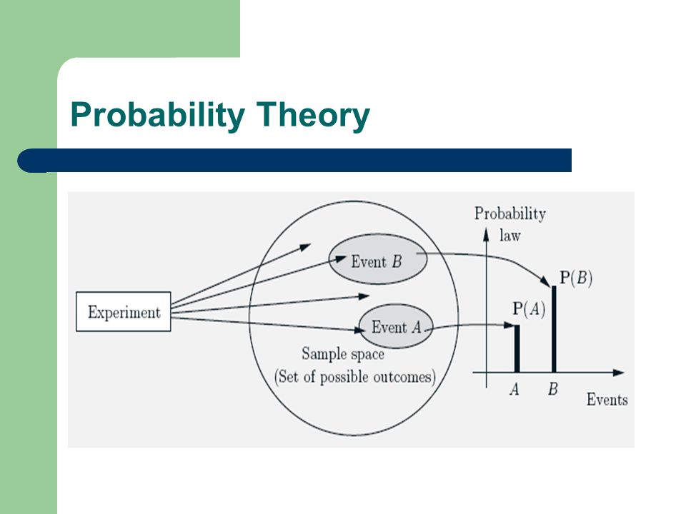
The set of all possible outcomes of an experiment is the sample space, denoted Ω. An event A is a (set of) possible outcomes of the experiment, and corresponds to a subset of Ω. Probability Theory
 possible outcomes of the experiment, and corresponds to a subset of Ω. Probability Theory.")
10
A probability law / measure is a function P(A) – with the argument A, – that assigns a value to A based on the expected proportion of number of times that event A is actually likely to happen. Probability Theory

12
Probability Theory: Axioms of Probability

13
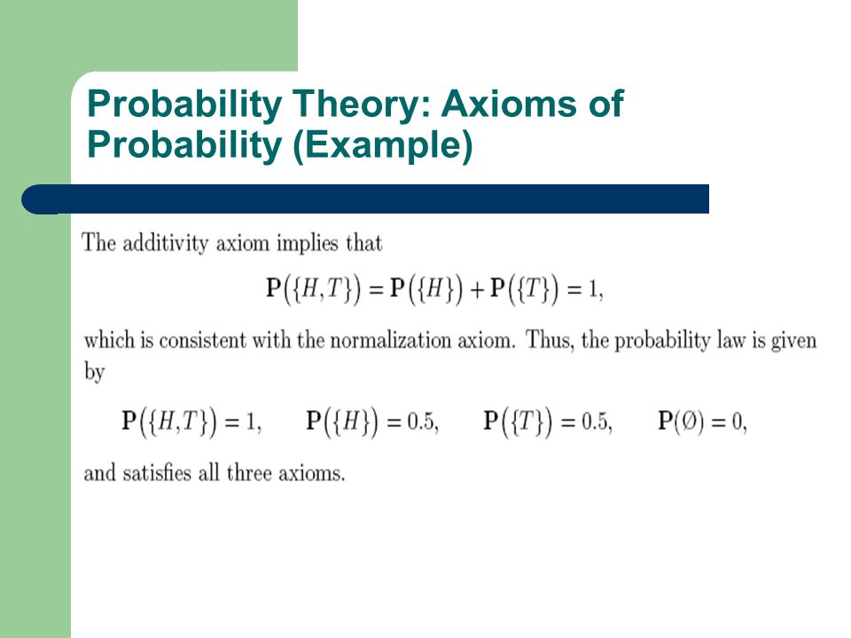
The probability function P(A) must satisfy the following: Probability Theory: Axioms of Probability
 must satisfy the following: Probability Theory: Axioms of Probability")
14
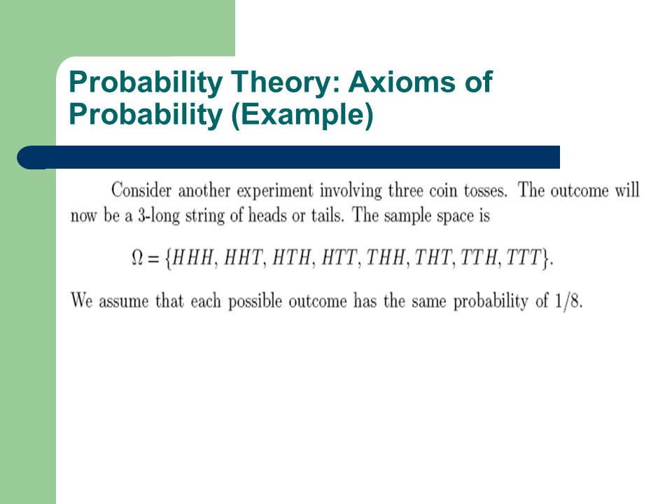
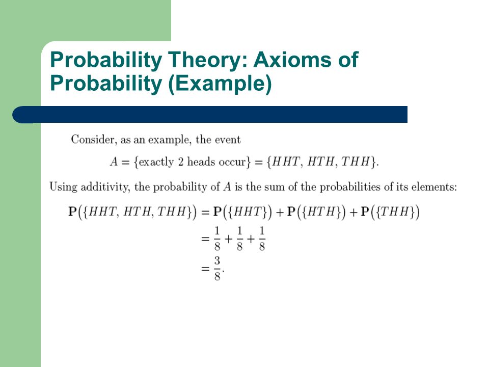
Probability Theory: Axioms of Probability (Example)
")
18
Probability Theory

19
In many probabilistic models, the outcomes are of a numerical nature, e.g., if they correspond to instrument readings or stock prices. In other experiments, the outcomes are not numerical, but they may be associated with some numerical values of interest. For example, if the experiment is the selection of students from a given population, we may wish to consider their grade point average. When dealing with such numerical values, it is often useful to assign probabilities to them. This is done through the notion of a random variable. Probability Theory: Random Variables

20
Briefly: – A random variable X is a function that maps every possible eventin the space Ωof a random experiment to a real number. Probability Theory: Random Variables

21
Random variables can discrete, e.g., the number of heads in three consecutive coin tosses, or continuous, the weight of a class member. Probability Theory: Random Variables

22
Random variables can – discrete, e.g., the number of heads in three consecutive coin tosses, or – continuous, the weight of a class member. Probability Theory: Random Variables

23
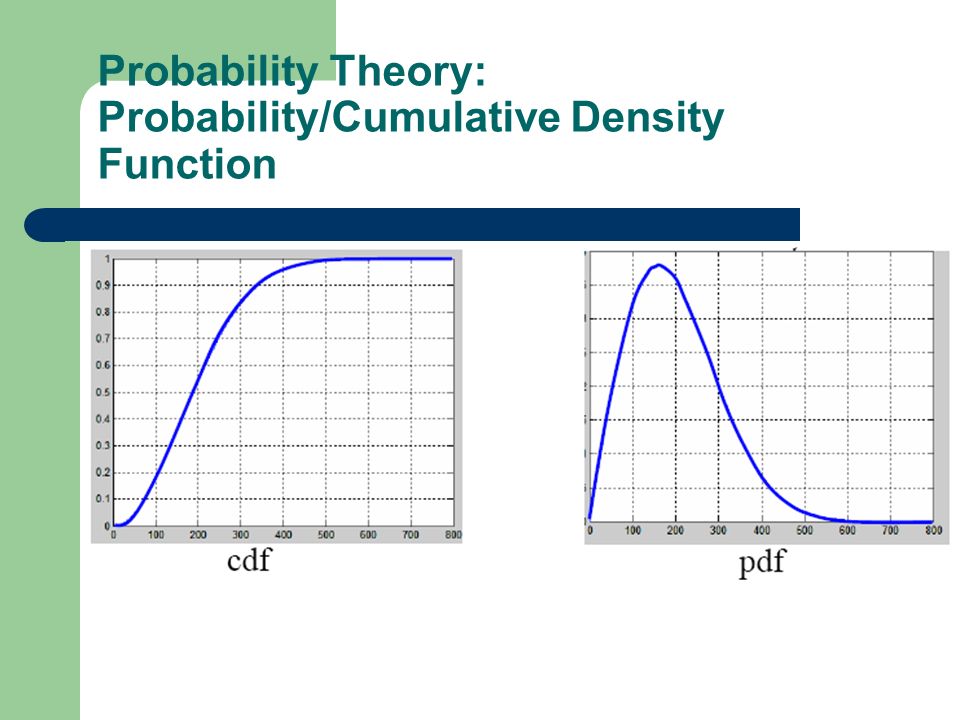
A probability mass (distribution) function is a function that tells us the probability of x, an observation of X, assuming a specific value. – P(X=x) The cumulative mass (distribution) function indicates the probability of X assuming a value less then or equal to x. – F(x) = P(X<=x) Probability Theory: Probability/Cumulative Mass Function
 The cumulative mass (distribution) function indicates the probability of X assuming a value less then or equal to x. – F(x) = P(X<=x) Probability Theory: Probability/Cumulative Mass Function.")
24
For continuos variables: – Probability Mass Function Probability Density function, – Cumulative Mass Function Cumulative Density Function Probability Theory: Probability/Cumulative Density Function

26
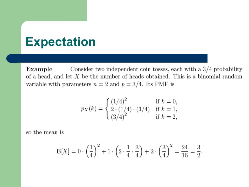
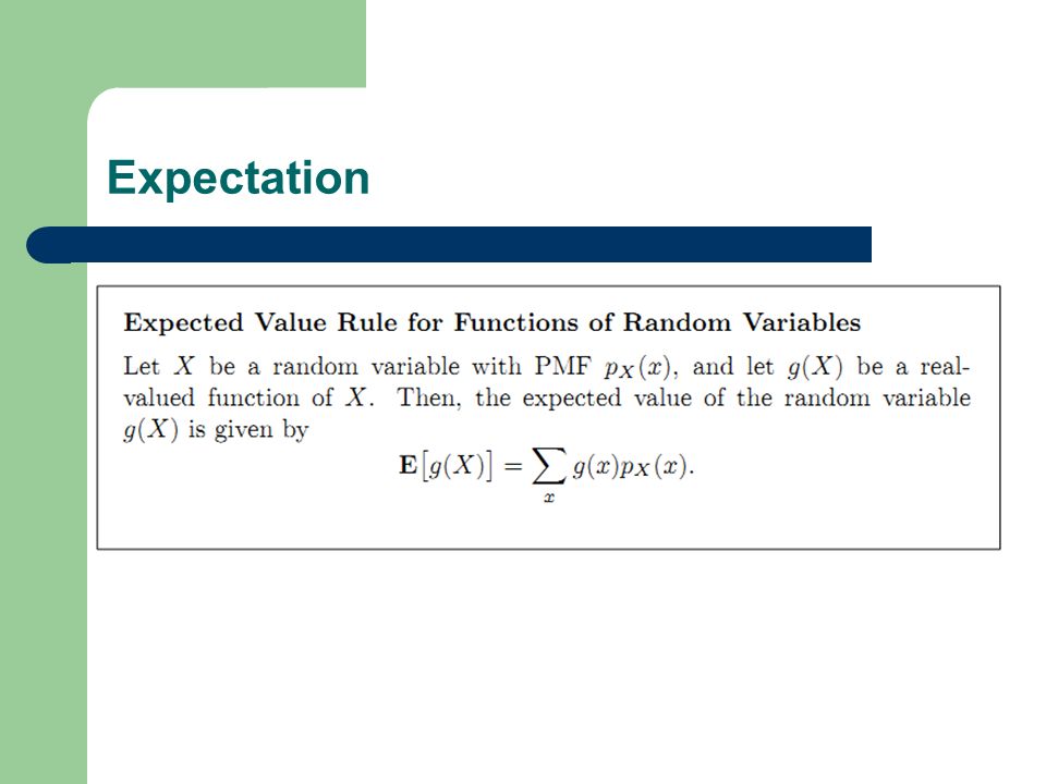
The PMF of a random variable X provides us with several numbers, the probabilities of all the possible values of X. It would be desirable to summarize this information in a single representative number. This is accomplished by the expectation of X, which is a weighted (in proportion to probabilities) average of the possible values of X. Expectation
 average of the possible values of X. Expectation.")
27
Example: – suppose you spin a wheel of fortune many times, – at each spin, one of the numbers m1,m2,..., mn comes up with corresponding probability p1, p2,..., pn, and – this is your reward from that spin. Expectation

28
Example: – What is the amount of money that you “expect” to get “per spin”? Expectation

29
Example: – Suppose that you spin the wheel k times, and that ki is the number of times that the outcome is mi. Then, the total amount received is m1k1 +m2k2 +· · ·+ mnkn. The amount received per spin is Expectation

30
Example: – If the number of spins k is very large, and if we are willing to interpret probabilities as relative frequencies, it is reasonable to anticipate that mi comes up a fraction of times that is roughly equal to pi: Expectation

31
Example: – Thus, the amount of money per spin that you “expect” to receive is Expectation

32
The expected value, or average, of a random variable X, whose possible values are {x1,…,xm} with respective probabilities p1,…,pm, is given as: Expectation

34
Moments of a random variable: Expectation

35
the variance, the average dispersion of the data from the mean Expectation

36
How ?

37
Expectation

38
Mean, second moment, variance ?

39
Expectation

40
The variance provides a measure of dispersion of X around its mean. An-other measure of dispersion is the standard deviation of X, which is defined as the square root of the variance Expectation

41
The standard deviation is often easier to interpret, because it has the same units as X. For example, if X measures length in meters, the units of variance are square meters, while the units of the standard deviation are meters. Expectation

43
Consider two discrete random variables X and Y associated with the same experiment. The joint PMF of X and Y is defined by Pairs of Random Variables

44
Joint probability also need to satisfy the axioms of the probability theory Everything that relate to X, or Y – individually or together – can be obtained from the P(x,y). In particular, the individual pmfs, called the marginal distribution functions can be obtained as Pairs of Random Variables

45
Random variables X and Y are said to be statistically independent, if and only if That is, if the outcome of one event does not effect the outcome of the other, they are statistically independent. For example, the outcome of two individual dice are independent, as one does not affect the other. Statistical Independence

46
Example

47
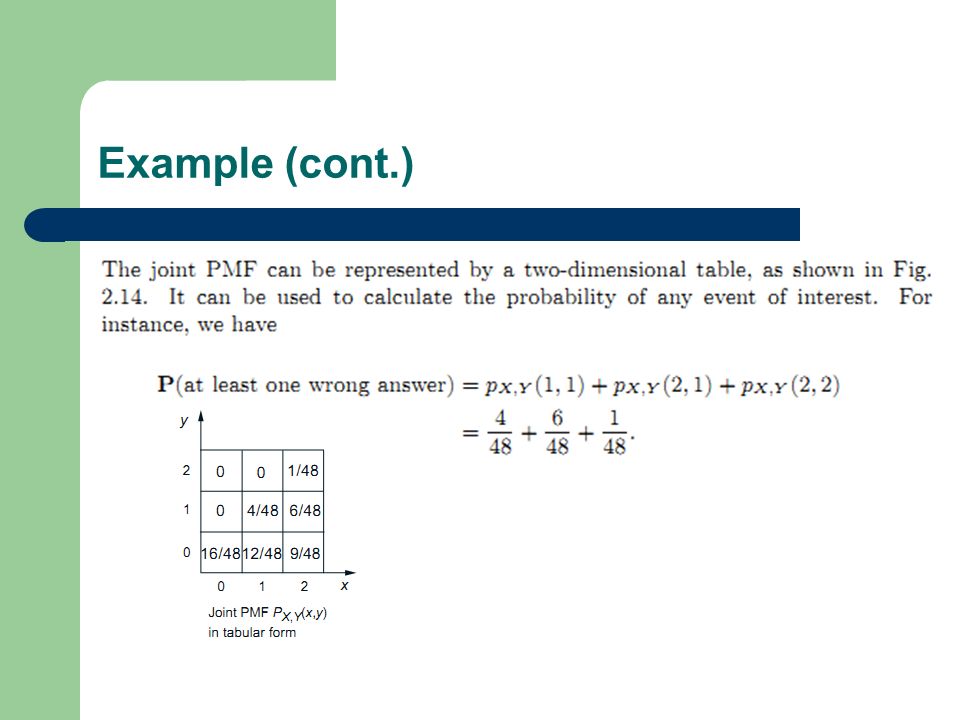
Example (cont.)
")
49
Expected values, moments and variances of joint distributions can be computed similar to single variable cases: Pairs of Random Variables

50
A cross-moment can also be defined as the covariance Covariance defines how the variables vary together as a pair – are they both increasing together, does one increase when the other decrease, etc Co-Variance

51
the covariance matrix, denoted by ∑ Co-Variance

52
If ρ=1, then the variables are identical, they move together, If ρ=-1, then the variables are negatively correlated, one decreases as the other increases at the same rate If ρ=0 the variables are uncorrelated. The variation of one, has no effect on the other. Correlation Coefficient

53
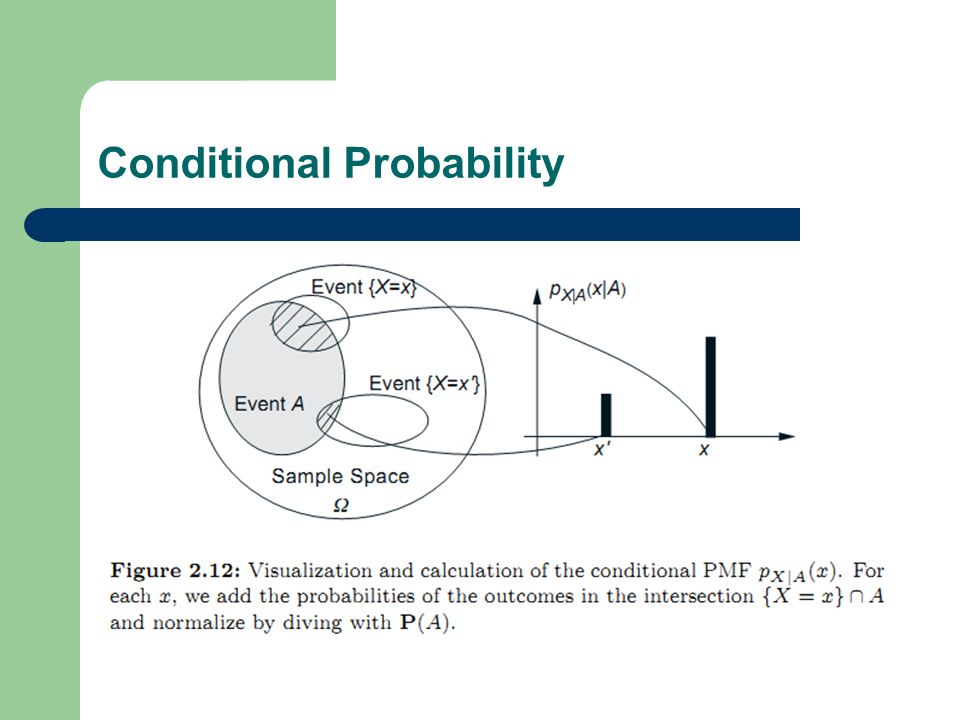
The conditional PMF of a random variable X, conditioned on a particular event A with P(A) > 0, is defined by Conditional Probability
 > 0, is defined by Conditional Probability")
54
A is a legitimate PMF. As an example, let X be the roll of a die and let A be the event that the roll is an even number. Then, by applying the preceding formula, we obtain Conditional Probability

56
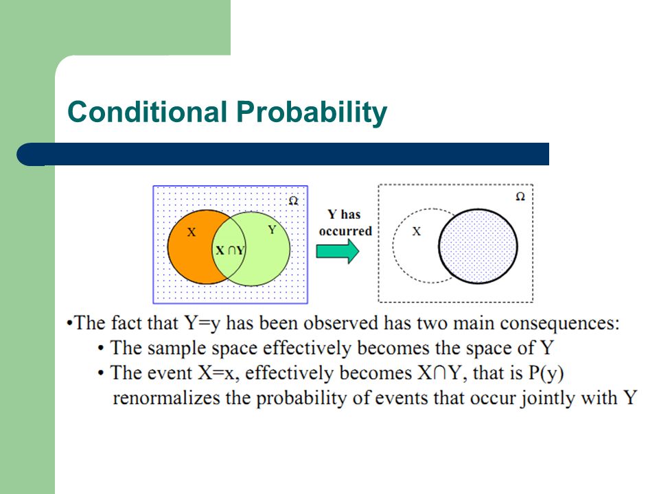
The conditional probability of X=x given the Y=y has been observed is given as Conditional Probability

58
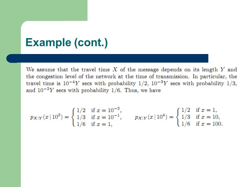
Example

59
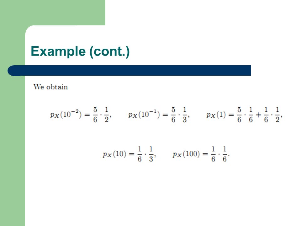
Example (cont.)
")
63
Law of Total Probability

64
Bayes Rule

66
Example

67
Many Dimensions

68
Random Vectors

69
Gaussian Distribution

70
Multivariate Gaussian Distribution

71
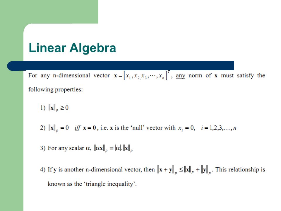
Linear Algebra x, u, v, w (bold face, lower case) d-dimensional column vector xi ith element of the vector X (bold face upper case) dxk dimensional matrix
 d-dimensional column vector xi ith element of the vector X (bold face upper case) dxk dimensional matrix")
72
Linear Algebra A linear combination of vectors is another vector: A collection of vectors are linearly dependent, if any one of them can be written as a linear combination of others with at least one non-zero scalar.

73
Linear Algebra A basis of V is a collection of linearly independent vectors such that any vector v in V can be written as a linear combination of these basis vectors. That if B={u1,u2,…,un} is a basis for V, than any v in V can be written as

74
Linear Algebra

77
An inner product in a vector space, is a way to multiply vectors together, with the result of this multiplication being a scalar.vector spacevectorsscalar More precisely, for a real vector space, an inner product satisfies the following four properties:real vector space

78
Linear Algebra

79
Orthogonality: Two vectors, x and y, in an inner product space, V, are orthogonal if their inner product, is zero.vectorsinner product spaceinner product

80
Linear Algebra Gradient: Jacobian:

81
Linear Algebra Hessian:

82
Linear Algebra Taylor expansions for vector valued functions:

83
References R.O. Duda, P.E. Hart, and D.G. Stork, Pattern Classification, New York: John Wiley, 2001. Dimitri P. Bertsekas and John N. Tsitsiklis, Introduction to Probability, 2nd Edition, 2008. Dimitri P. BertsekasJohn N. Tsitsiklis Robi Polikar, Rowan University, Glassboro, Pattern Recognition Course Materials, 2001.

Similar presentations


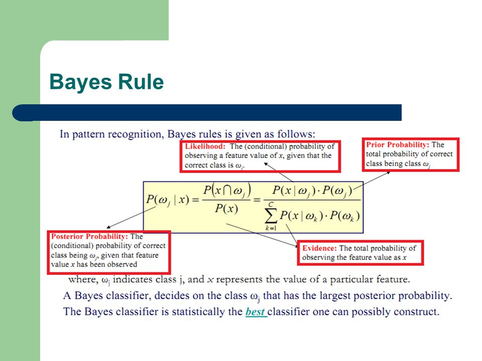


 and the class- conditional probabilities P(x|wi)>")


