1. Osyczka Andrzej Krenich Stanislaw Habel Jacek Department of Mechanical Engineering, Cracow University of Technology, 31-864 Krakow, Al. Jana Pawla II 37, Poland email: osyczka@mech.pk.edu.pl, krenich@mech.pk.edu.pl, habel@mech.pk.edu.pl

2. Contents  Introduction  General description of EOS  Some methods from EOS  Bicriterion method  Constraint tournament method for single and multicriteria optimization  Indiscernibility interval method  Features of EOS  Running EOS  Applications examples  Spring design automation  Robot gripper mechanism design  Network optimization

3. Evolutionary Optimization System (EOS) is designed to solve single and multicriteria optimization problems for nonlinear programming problems, i.e. for the problems formulated as follows: find x * = [x 1 *, x 2 *,..., x I * ] which will satisfy the K inequality constraints g k (x)  0 for k = 1, 2, …, K (1) and the M equality constraints h m (x) = 0 for m = 1, 2, …, M (2) and optimize the vector of objective functions: f(x * ) = [f 1 (x), f 2 (x),...,f N (x)] (3) where: x = [x 1,x 2,...,x I ] is the vector of decision variables, For single criterion optimization problems instead of the vector function f(x) we have the scalar function f(x) which is to be minimized. The system is coded in the ANSI C language. Introduction

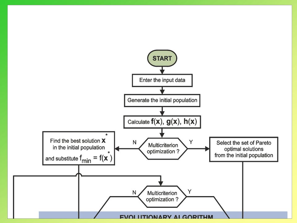
4. General description of EOS

5. The main idea of the proposed method consists in transforming the single criterion optimization problem into the bicriterion optimization problem with the following objective functions: Some methods from EOS - Bicriterion method where: G k is the Heaviside operator such that G k = -1 dla g k (x)  0, G k = 0 dla g k (x)  0. f 2 (x) = f(x) - the objective function that is to be minimized The minimum of f 1 (x) is known and equals zero. The function f 1 (x) will achieve its minimum for any solution that is in the feasible region.

6. Some methods from EOS - Bicriterion method Sets of Pareto solutions for a numerical example

7.  If both chromosomes are not in the feasible region the one which is closer to the feasible region is taken to the next generation. The values of the objective function are not calculated for either of chromosomes.  If one chromosome is in the feasible region and the other one is out of the feasible region the one which is in the feasible region is taken to the next generation. The values of the objective function are not calculated for either chromosome.  If both chromosomes are in the feasible region, the values of the objective function are calculated for both chromosomes and the one, which has a better value of the objective function is taken to the next generation. In this method the tournament between two chromosomes is carried out in the following way: Some methods from EOS - Constraint Tournament Method for Single Criterion Optimization The constraint violation function can be evaluated as follows: where: G k is the Heaveside operator such that G k =0 for and G k =1 for

8. The feasible domain 653214 5 41 Feasible solution f(x 5,t ) < f(x 6,t ) Some methods from EOS - Constraint Tournament Method for Single Criterion Optimization

9. Some methods from EOS - Constraint Tournament Method for Multicriteria Optimization The feasible domain 653214 5 41 6 Feasible solution

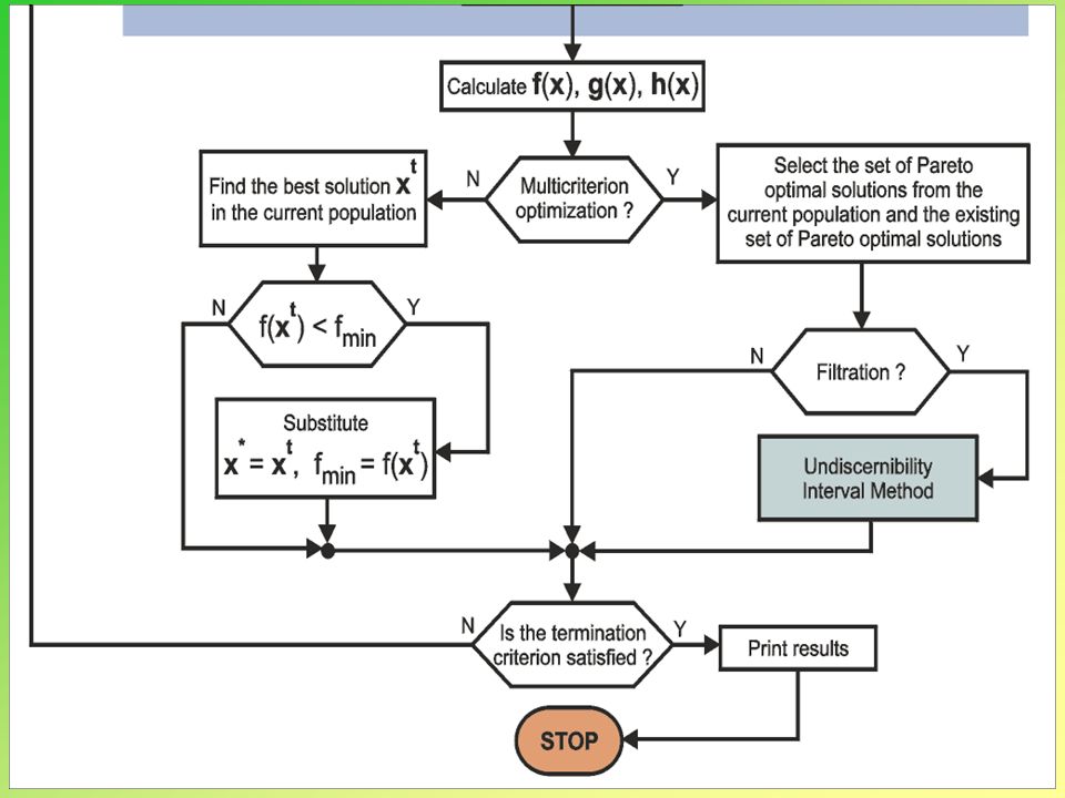
10. The steps of the method are as follows: Step 1. Set t = 1, where t is the number of the currently run generation. Step 2. Generate the set of Pareto optimal solutions using any evolutionary algorithm method. Step 3. Is the criterion for filtration the set of Pareto solutions satisfied? If yes, select the representative subset of Pareto solutions using the indiscernibility interval method and go to step 4. Otherwise, go straight to step 4. Step 4. Set t = t + 1 and if t  T, where T is the assumed number of generations, go to step 2. Otherwise, terminate the calculations. Some methods from EOS - Indiscernibility interval method The idea of the method consists in reducing the set of Pareto optimal solutions using indiscernibility interval method after running a certain number of generations.

11. Graphical illustration of the indiscernibility interval method Some methods from EOS - Indiscernibility interval method

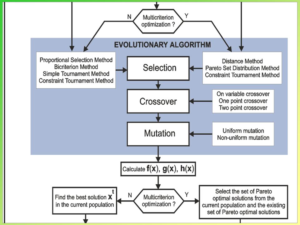
12. Features of EOS For both single and multicriteria optimization methods the following models can be solved: with continuous decision variables, with integer decision variables, with discrete decision variables, with mixed continuous – integer decision variables, with mixed continuous – discrete decision variables. In EOS chromosomes can have: binary representation, real number representation, Grey coding representation. Crossover operations can be performed as follows: one point crossover, two point crossover, variable point crossover. Mutation operations can be performed as follows: uniform mutation, non-uniform mutation.

13. Running EOS – The Main Control Window

14. Running EOS – The User Function File Window

15. Running EOS – The Output File Window

16. 1) Spring design automation 2) Robot gripper mechanism design 3) Network optimization Applications examples

17. Examples of Spring Design Automation - Helical Spring Design x2x2 x1x1 x3x3 Scheme of the spring The vector of decision variables is x 1 – wire diameter of the spring [mm] x 2 – meancoil diameter of the spring [mm] x 3 – length of the spring [mm] x 4 – number of active coils [–] The objective function is the volume of the spring The constraints are: 1)shear stress constraint, 2)stiffness of the spring constraint, 3)clearance between coils constraint, 4)buckling constraint, 5)geometric constraints, The optimization model is considered a discrete type, with the following sets of possible values: X 1 = {0.5, 0.63, 0.8,..., 6.3, 8.0, 10.0 }, X 2 = {1,2,3,4,...,60,61,62,...,300}, X 3 = {1,2,3,...,50,51,52,...,600}, X 4 = {1.5,2.5,...,49.5}

18. Helical Spring Design - Numerical Results Example no. 1 Example no.2 Material of the spring 45S70S3 Compression force P [N] 1850580.8 Stiffness of the spring s[N/mm]/ Deflection of the spring d[mm] 20.55 62 Type of the springNon running running The best results obtained using the automation design method Results obtained using a general design procedure f(x)84 989.59 100 023.18 x1x1 8.0 x2x2 63.060.0 x3x3 159. 0196. 0 x4x4 7.59.5 Table 2. Results of automation of design of the spring: example1 Table 1. Input data of the spring design problem

19. Optimization model of the robot gripper Vector of decision variables: x = [ a, b, c, e, f, l,  ] T, where a, b, c, e, f, l, are dimensions of the gripper and  is the angle between the elements b and c. Constraints: 1.On the basis of the geometrical dependencies and dependencies between the forces several constraints are built and used. 2.They depend also on the stages of the optimization process. Objective functions: 1.f 1 (x) - the difference between maximum and minimum griping forces for the assumed range of the gripper ends displacement, 2.f 2 (x) - the force transmission ratio between the gripper actuator and the gripper ends, 3.f 3 (x) - the shift transmission ratio between the gripper actuator and the gripper ends, 4.f 4 (x) - the length of all the elements of the gripper, 5.f 5 (x) - the maximal force in the joints, 6.f 6 (x) - the efficiency of the gripper mechanism.

20. Multistage process of the robot gripper optimization Ordering of the criteria: Constraints: Stage 1: The set of Pareto optimal solutions

21. Multistage process of the robot gripper optimization Constraints: Stage 2: The set of Pareto optimal solutions

22. Multistage process of the robot gripper optimization Constraints: Stage 5: The set of Pareto optimal solutions

23. Tabela 7.22. Przykładowe rozwiązania ze zbioru Pareto uzyskane w etapie 5 optymalizacji

24. Network optimization An example of network which has no Markow property An example of network which has Markow property

25. Osyczka Andrzej Krenich Stanislaw Habel Jacek Department of Mechanical Engineering Cracow University of Technology, 2002 Thank You for Your Attention