1. Thermal Analysis

2. 1. Introduction
 Thermal Analysis is the term applied to a group of methods and techniques in which chemical or physical properties of a substance, a mixture of substances or a reaction mixture are measured as function of temperature or time, while the substances are subjected to a controlled temperature programme.

3. * Introdcution to Thermal Analysis, M.E. Brown -- Chapman and Hall
* Thermal Analysis - Techniques and Applications, ed. E.L. Charsley and S.B. Warrington -- Royal Society of Chemistry
* Thermal Analysis of Materials, Robert F. Speyer –Marcel Dekker, Inc.
References:

4. The following table is a list of the main thermal analysis methods:

5. While carrying out these measurements, the furnace atmosphere can either be static air or a continuous flow of gas (purging). Examples are inert conditions (nitrogen) to inhibit oxidation, or reducing condition (e.g. purging hydrogen), etc.

6. General thermodynamic relationships
Thermal analyses are usually run under conditions of constant pressure, the underlying thermodynamic equation is the Gibbs-Helmholtz expression:
G0=H0-TS0
where G=free energy of the system, H=enthalpy of the system, S=entropy of the system, T=temperature in kelvins
The general chemical reaction
aA+bBcC+dD
Is spontaneous as written if G<0, is at equilibrium if G=0, and does not proceed if G >0.
Thermal analysis involves the monitoring of spontaneous reaction.

7. Differentiating the Gibbs-Helmholtz equation with respect to temperature (assuming S and H not vary with temperature):
Show how to move from a stable situation (G>>0) to one where reaction will occur.
S>0, an increase in temperature cause G<0,
S<0, decreasing the temperature will achieve the desired spontaneous reaction.
Once the reaction is made to occur, thermal analysis may be used to detect the process, yielding different and complementary information.

8. 2. Thermogravimetry
Thermogravimetric analysis (TG) is the study of weight changes of a specimen as a function of temperature. The technique is useful strictly for transformations involving the absorption or evolution of gases from a specimen consisting of a condensed phase.
A plot of mass versus temperature (thermogravimetric curves or TG curves) permits evaluation of thermal stabilities, rate of reaction, reaction processes, and sample composition.
* Measurements of changes in sample mass with temperature are made using thermobalance. The balance should be in a suitably enclosed system so that the atmosphere can be controlled.

9. General considerations
Suitable samples for TG are solids that undergo one of the two general types of reaction:
Reactant(s)  Product(s)+Gas (a mass loss)
Gas+Reactant(s)  Product(s) (a mass gain)
Processes occuring without change in mass (e.g., the melting of a sample) obviously cannot be studied by TG.

10. 2.1 Instrumentation
LINSEIS L81

11. Thermogravimetric instrumentation should include several basic components to provide the flexibility necessary for the production of useful analytical data:
A balance,
A heating device,
A unit for temperature measurement and control,
A means for automatically recording the mass and temperature changes,
A system to control the atmosphere around the sample.

12. 2.1.1 The Thermobalance
Two typical designs of the thermobalance are shown in the following:

13. Balances must remain precise and accurate continuously under extreme temperature and atmosphere conditions, and should deliver a signal suitable for continuous recording.
*   Null-deflection weighing mechanisms are favoured in TG as they ensure that the sample remains in the same zone of the furnace irrespective of changes in mass.
*   Sensitivity of balance  1g for a 1g maximum load balance.
*   The output weight signal may be differentiated electronically to give a derivative thermogravimetric curve (DTG)

14. 2.1.2 The Heating Chamber
The furnace is normally an electrical resistive heater;
Some basic requirements of the heating chamber are :
be non-inductively wound
be capable of reaching 100 to 200°C above the maximum desired working temperature
have a uniform hot-zone of reasonable length
reach the required starting temperature as quickly as possible
not affect the balance mechanism through radiation or convection
In order to overcome the problem of possible temperature gradient, infrared or microwave radiation have been used in some equipment.
infrared heating : use halogen lamp, temperature up to 1400°C, heating rate can be as high as 1000°C/min, accuracy is about ±0.5°C.
Microwave heating : large sample can be used because uniform heating generated within sample but temperature measurement and power control are difficult.

15. Constant heating rate

16. Constant heating rate: lag behind of the sample temperature
During heating a temperature difference between the furnace and the sample temperature appears which means that the sample temperature lags always behind the furnace temperature.
Measurement of the melting point of Di-tert.-biphenyle at different heating rates.

17. Gradual raise of temperature
Thermal equilibrium is better reached by gradual raise of the temperature.

18. 2.1.3 The atmosphere
Sort, pressure and flow rate of the gas in the sample chamber influence the following parameters:
Sample reaction
Sample reactions with the gas (oxidation in the presence of oxygen).
Heat transitions
Different heat conductivity of the gases used in an experiment.
Buoyancy and current effects
Different density and flow rate of the gases used in an experiment.
For all thermoanalytical investigations it is very important to report the sort, the pressure and the flow rate of the gases used in the experiment.

19. Thermal decomposition temperatures for CaCO3 in different gas atmospheres

20. *  Thermbalance are normally housed in glass or metal system to allow for operation at pressures ranging from high vacuum (< 10-4 Pa) to high pressure (>3000 kPa) of inert, oxidizing, reducing or corrosive gases.
*  Care must be taken to correct for buoyancy arising from the lack of symmetry in the weighing system
*  Thermal convection is responsible for noise in the signal of TG. The use of dense carrier gases at high pressures in hot zones with large temperature gradients give the most noise. Fitting of convoluted baffles was found to be most successful in reducing thermal convection.

21. 2.1.4 The sample
Sample form, defect content, porosity and surface properties has influence to the behaviour on heating, e.g. single crystal sample give different response from powdered sample
Large sample size cause problems like heat transfer, and gas exchange with the surrounding is reduced; in general, the use of small (~ 20 mg) specimen is preferable if sensitivity of balance permits
Sample should be powdered and spread thinly and uniformly in the container

22. Crucibles

23. Decomposition temperatures of CaCO3 as function of crucibles

24. 2.1.5 Temperature measurement and calibration
Platinum resistance thermometers or thermocouples are used for temperature measurement.
Large difference between sample temperature (Ts) and furnace temperature (Tf) can exist, sometime as high as 30°C. Calibration is thus needed.
The difference or lag is more marked when operating in vacuum or in fast flowing atmosphere and with high heating rate.

25. Temperature calibration for small furnace can be done by making use of the melting point or Curie points of a range of metals and alloys.
A series of high purity wires may be suspend in the region where the specimen crucible would normally be located. If the furnace temperature is slowly raised through the melting point of a particular wire, a significant weight loss will be recorded when the wire melts.
A series of fusible wire, such as : indium (156.63°C), lead (327.5°C), zinc (419.58°C), aluminium (660.37°C), silver (961.93°C), and gold ( °C) should give a reasonable calibration curve.
hanger of sample pan
furnace
different metal wires
thermocouple

26. Calibration can also be done by placing a series of ferromagnetic materials in the specimen basket and a magnet below or above it, external to the furnace. When each material goes through its Curie temperature (ferro- to paramagnetic transition), a sharp ‘weight’ change will be indicated.

27. 2.2 Interpretation of TG and DTG curves
The sample undergoes no decomposition with loss of volatile products over the temperature range shown but solid phase transformation, melting ,etc can not be detected by TG,
The rapid initial mass loss is characteristic of desorption or drying. If it is true, then re-run the sample should result in type (i) curves,
Single stage decomposition,
Multi-stage decomposition with relatively stable intermediates : provide information on the temperature limit of stability of reactants and intermediate products and also stoichiometry,
Multi-stage decomposition with no stable intermediate product. However heating-rate effect must be considered. At low heating rate, type (v) resemble type (iv). At high heating rate, type (iv) and (v) resemble type (iii) and lose all the details,
Gain in mass due to reaction with atmosphere, e.g. oxidation of metals,
Oxidation product decompose again at higher temperature; this is not often encountered.
Resolution of stages can be improved by recording DTG or by digital differentiation of TG data.

28. 2.3 Preparing the measurement
General advices:
Exact characterization of the starting materials (purity, grain size)!
Large amount of the starting material for repeated and further measurements
Removal of absorbed water by drying (m must be constant)
Use samples with narrow grain size distribution (Sieving)
For measurement in vacuum no sample with a grain size below 60 mesh (0.25 mm) (a part of the sample can be lost)

29. 2.4 Applications of TG
only for studying thermal events accompanied by mass change
provide valuable information for desorption, decomposition and oxidation. e.g. dehydration of CuSO4·5H2O
TG curve for CuSO45H2O
TG curve for CaSO42H2O at different water-vapour pressure

30. Three factors should be noted when you get a TG curve: General shape,
knowledge of thermal stability can give information on problems like the hazards of storing explosives, shelf life of drugs, etc.
TG curves can also be used for 'fingerpring' purpose.
The thermal balance in a TG equipment can also be used to measure vapour pressure of a sample and magnetic susceptibility, etc.
ATTN:
Three factors should be noted when you get a TG curve:
General shape,
The particular temperatures at which changes in mass occur (severely affected by many experimental conditions),
The magnitudes of the mass changes (much more use directly related to the specific stoichiometries of the reactions, independent of the many factors that affect the shape of the curves. Can be used for precise quantitative analysis).

31. Analytical calculations
Under controlled and reproducible conditions, quantitative data can be extracted from the relevant TG curves. Most commonly, the mass change is related to sample purity or composition.
Example: A pure compound may be either MgO, MgCO3, or MgC2O4. A thermogram of the substance shows a loss of 91.0 mg from a total of mg used for analysis. What is the formula of the compound? The relevant possible reactions are
MgO  No reaction
MgCO3  MgO+CO2
MgC2O4  MgO+CO2+CO
Solution: % Mass loss Sample=(91.0/175.0)(100%)=52.0
% Mass loss if MgCO3=(44/84.3)(100%)=52.2
% Mass loss if MgC2O4=((44+28)/112.3)(100%)=64.1
If the preparation was pure, the compound present is MgCO3.

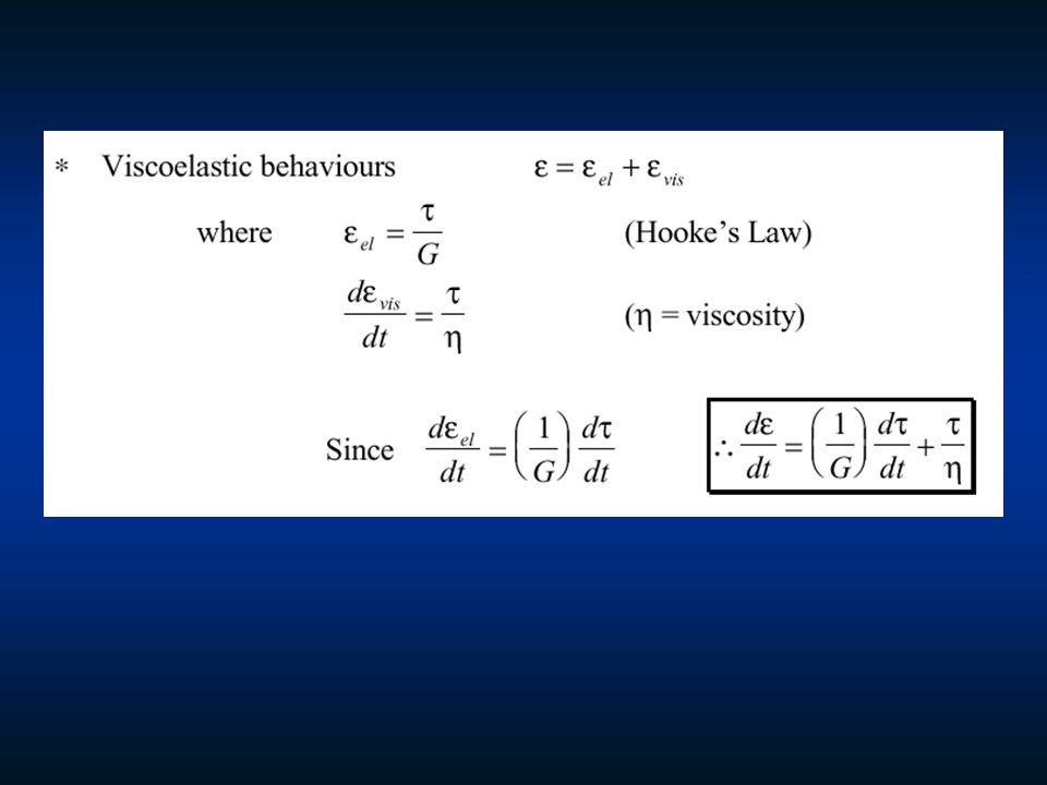
32. 3. Dynamic Mechanical Analysis
3.1 Viscoelastic Properties of Polymers 
* A polymer may exhibit mechanical behaviour characteristic of either an elastic solid or a viscous liquid, depending upon temperature, in relation to the glass-transition temperature (Tg) of the polymer and the time scale of the deformation. 
* Two extremes types of stress-strain curves are those for elastic solid ( , Hooke’s law) and fluid (  d/dt, Newton’s law) 
relationship between moduli: E = 3B(1-2) = 2(1+)G
E: Young’s modulus; B: bulk modulus; G: shear modulus; : Poisson’s ratio

35. For polymer, if d/dt = constant, a curve like the following will be observed

36. 3.2 Periodic stress and DMA
 *  In DMA, the sample is subjected to a sinusoidally varying stress of angular frequency . The strain is also sinusoidal but out of phase with the stress by an angle  due to internal damping effects.

37. The response of the sample to this treatment can provide information on the stiffness of the material (quantified by its elastic moduli) and its ability to dissipate energy (measured by its damping). For a viscoelastic material, the strain resulting from the periodic stress will also be periodic, but will be out of phase with the applied stress owing to energy dispersion as heat, or damping.
If an elastic sample is vibrated over a range of frequencies and the amplitude of vibration is measured, the resonance frequency is that which produces a maximum in a plot of amplitude against frequency. Young's modulus (of elasticity), E, is related to the square of the resonance frequency, Vr.
where c is a constant, L is the sample length between clamps, d is the sample thickness and  is the sample density.

38. 3.3 The resonance frequency
If a sample is vibrated over a range of frequencies and the the amplitude of vibration can be measured, the resonance frequency is that which produces a maximum in a plot of amplitude against frequency. Modulus is related to the resonance frequency.
Free oscillation with damping
Damping: log10(A1/A2)=log10(A2/A3)

39. For elastic materials, the modulus E is simply the constant ratio between the stress and the resulting strain, but for viscoelastic materials, the modulus is a complex quantity:
E* = E' + iE"
where E' is the storage modulus or in-phase component and E" is the loss modulus or out-of-phase component. The ratio E" / E' is the tangent of the phase angle, .

40. For this forced-vibration situation, complex variables (i. e
* For this forced-vibration situation, complex variables (i.e. ) is used for analysis The modulus can also be written as G* = G + iG where G is called the storage modulus and G is called the loss modulus.

41. *  The outputs of the test are usually temperature variation plots of either tan , G and/or G or some other combinations of these parameters.
DMA response of polystyrene cross-linked with 2% divinyl benzene
DMA spectrum of polysulfone.
o : storage_modulus;  : loss-modulus. (Tg 480K)

42. 3.3 Apparatus
* The sample is set in cyclic tensile load, a linear variable differential transformer (LVDT) is used to monitor the frequency and the amplitude of vibration.
* The preset oscillation amplitude is maintained by a feedback control loop and the driving force required to do so is a measure of the energy dissipation of the sample

43. 3.4 Applications
* change in E (or G) indicate changes in rigidity and hence strength of the sample (cure behaviour)
*damping measurements give practical information on glass transitions, change in crystallinity, the occurrence of cross-linking and also show up the features of polymer chains
*  damping information can be useful in studies of vibration dissipation impact resistance and noise abatement.
* Stress relaxation behaviour of polymer

44. Typical DMA results on two different samples of polyethylene
(a) Linear polyethylene
(b) branched polyethylene.
The damping curve for linear polyethylene (a) shows peaks at -95°C and 65°C. The lower temperature peak has been attributed to long chain (-CH2-)n crankshaft relaxations in the amorphous phase and the higher temperature peak to similar motion in the crystalline phase. The temperatures and relative sizes of the two peaks can be related to the degree of crystallinity of the sample.
The damping curve for branched polyethylene (b) has features at -112°C, -9°C and 45°C. The -112°C and 45°C peaks are explained as above, while the -9°C peak is attributed to (-CH3) relaxations in the amorphous phase.

45. The thermal behaviour of styrene-butadiene-rubber (SBR)
Various formulations of SBR are used in tyre manufacture. Different styrene-butadiene ratios may be used, or different butadiene isomers, or different additives e.g. carbon black. A high cis-butadiene content (a) lowers the glass transition temperature, Tg, (to as much as -110°C compared to -50°C) giving greater flexibility at low temperatures. The addition of carbon black (c) increases the modulus of elasticity. The Tg is also slightly increased. The complex damping curve at low temperatures indicates polymer-carbon black interactions and may lead to adverse properties e.g. heat build-up.

46. 4. Differential Scanning Calorimetry
In power-compensated DSC, the sample and a reference material are maintained at the same temperature throughout the controlled temperature programme. The difference in the independent energy supplies to the sample and the reference is then recorded against the programme temperature
DSC can be used to study heats of reaction, kinetics, heat capacities, phase transitions, thermal stabilities, sample composition and purity, critical points, and phase diagrams.

47. Circuitry of a DSC
Two separate heating circuits:
The average-heating controller
(the temperatures of the sample (Ts) and reference (Tr) are measured and averaged and the heat output is automatically adjusted to increase the average temperature of the sample and reference in a linear rate)
Differential-heating circuit
(monitor the difference in Ts and Tr, and automatically adjust the power to either the reference or sample chambers to keep the temperatures equal)
x-axis: temperature, y-axis: the difference in power supplied to the two differential heater (calories per unit time).

48. DSC trace of poly(ethylene terephthalate-co-p-oxbenzoate)
·  Thermal events in the sample appear as deviation from the DSC baseline, in either an endothermic or exothermic direction (marked on DSC curves). In DSC, endothermic responses are usually represented as being positive, i.e. above the base line.
Power difference
DSC trace of poly(ethylene terephthalate-co-p-oxbenzoate)

49. 4.2 Sample containers and sampling
DSC cell

50. * T<500°C : usually contained in aluminium sample pans which can be sealed either by crimping or by cold-welding for holding volatile samples
* T>500°C : use quartz, alumina (Al2O3), gold or graphite pans
* the reference material in most DSC applications is simply an empty sample pan
* purging of gas into the DSC sample holder is possible, e.g. N2, O2, etc.
* the mass of (sample+pan+lid) should be recorded before and after a run so that further information about the processes can be deduced

51. The reference sample
For all difference methods (DTA, DSC) reference samples like Al2O3 are needed to ensure that the heat flow from the furnace to the sample and from the furnace to the reference sample is identical!
The thermal behavior of the reference sample is included in the measured signal.
Requirements for the reference sample:
Known temperature behavior
No discontinuity in the temperature curve
If possible a similar thermal behavior as the sample (similar heat capacity)
For small weights of the sample and when no precise measurements are required an experiment without a reference sample is possible.
In such case an empty crucible can be used as reference.

52. 4.3 Interpretation of DSC curves
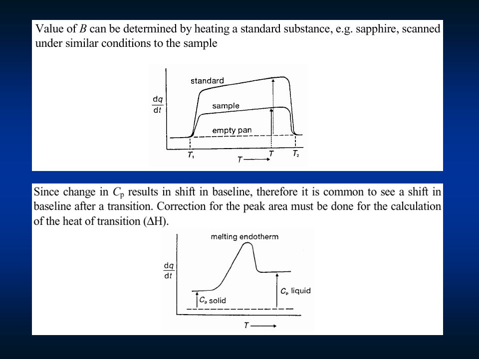
* aim at correlating the features recorded with the thermal events taking place in the sample
* after baseline correction, the peak area is proportional to enthalpy change,
where K is a constant and m is the mass of the sample
K can be obtained by melting a known amount of a pure metal

54. Heating and cooling curves for a partially crystallized polymer.
reversibility can be monitored by cooling and reheating
Heating and cooling curves for a partially crystallized polymer.

56. 4.4 Applications
4.4.1 Measurement of heat capacity
G = H - TS

58. 4.4.2 Measurement of thermal conductivity
* The temperature at the bottom of the sample (T1) is measured via the output of the DSC, while the temperature at the top of sample is measured with a separate thermocouple in the contact rod.

59. * The DSC cell is brought to the desired measurement temperature, T, and when the output to the recorder is steady with time, the temperature difference across the sample Ts and the displacement of baseline, hs, is recorded. The same is then go through for a standard calibrant, e.g. a standard glass.
where Ri = recorder sensitivity
li = length of sample/calibrant
di = diameter of sample/calibrant

60. 4.4.3 Determination of phase diagrams
melting point can be determined from the DSC curve

61. * Melting point of pure components are easily determined
* DSC curves for slow cooling of mixture

62. * If heating is done instead of cooling, the curve should ideally be endothermic mirror image of that shown and the problem of supercooling is avoided.
* From a series of this kind of curves, a phase diagram can be constructed.

63. 4.4.4 General Applications
* Temperature and enthalpy changes for the thermal events
enthalpy  area of peak after baseline correction
Corresponding TG curve

64. * Detection of solid-solid phase transition and the measurement of H for these transitions
DSC curve of carbon tetrachloride

65. Tracing the ferromagnetic to paramagnetic transformation.
Most rewarding applications is in study of polymer
Most solid polymers are formed by rapid cooling to low temperatures (quenching) are thus in glassy state; by heating above Tg, glass transition, with change in cp but no change in enthalpy, is observed, therefore no peak is observed, only discontinuity results

66. degradation or oxidation of polymers can be study with DSC in isothermal mode
for recycling plastics, identification is important and DSC curves provide 'fingerprint'of the materials.