Download presentation
Presentation is loading. Please wait.

1
Class 4 Ordinary Least Squares SKEMA Ph.D programme 2010-2011 Lionel Nesta Observatoire Français des Conjonctures Economiques Lionel.nesta@ofce.sciences-po.fr

2
Introduction to Regression Ideally, the social scientist is interested not only in knowing the intensity of a relationship, but also in quantifying the magnitude of a variation of one variable associated with the variation of one unit of another variable. Regression analysis is a technique that examines the relation of a dependent variable to independent or explanatory variables. Simple regression y = f(X) Multiple regression y = f(X,Z) Let us start with simple regressions
 Multiple regression y = f(X,Z) Let us start with simple regressions.")
3
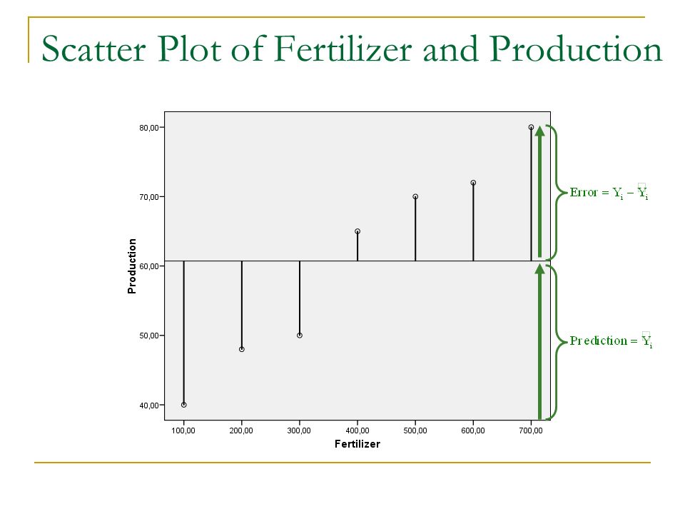
Scatter Plot of Fertilizer and Production

8
Objective of Regression It is time to ask: “What is a good fit?” “A good fit is what makes the error small” “The best fit is what makes the error smallest” Three candidates 1.To minimize the sum of all errors 2.To minimize the sum of absolute values of errors 3.To minimize the sum of squared errors

9
To minimize the sum of all errors X Y – – + X Y – + + Problem of sign

10
X Y +3 To minimize the sum of absolute values of errors X Y –1 +2 Problem of middle point

11
To minimize the sum of squared errors X Y – – + Solve both problems

12
ε ε²ε² Overcomes the sign problem Goes through the middle point Squaring emphasizes large errors Easily Manageable Has a unique minimum Has a unique – and best - solution To minimize the sum of squared errors

13
Scatter Plot of Fertilizer and Production

14
Scatter Plot of R&D and Patents (log)
")
18
The Simple Regression Model y i Dependent variable (to be explained) x i Independent variable (explanatory) α First parameter of interest Second parameter of interest ε i Error term
 x i Independent variable (explanatory) α First parameter of interest Second parameter of interest ε i Error term")
19
The Simple Regression Model

20
ε ε²ε² To minimize the sum of squared errors

21
ε ε²ε²

22
Application to SKEMA_BIO Data using Excel

24
Interpretation When the log of R&D (per asset) increases by one unit, the log of patent per asset increases by 1.748 Remember! A change in log of x is a relative change of x itself A 1% increase in R&D (per asset) entails a 1.748% increase in the number of patent (per asset).
 entails a 1.748% increase in the number of patent (per asset)..")
25
OLS with STATA Stata Instruction : regress (reg) reg y x 1 x 2 x 3 … x k [if] [weight] [, options] Options : noconstant : gets rid of constant robust : estimates robust variances, even with heteroskedasticity if : selects observations weight : Weighted least squares
![OLS with STATA Stata Instruction : regress (reg) reg y x 1 x 2 x 3 … x k [if] [weight] [, options] Options : noconstant : gets rid of constant robust : estimates robust variances, even with heteroskedasticity if : selects observations weight : Weighted least squares](http://images.slideplayer.com/21/6308080/slides/slide_25.jpg "OLS with STATA Stata Instruction : regress (reg) reg y x 1 x 2 x 3 … x k [if] [weight] [, options] Options : noconstant : gets rid of constant robust : estimates robust variances, even with heteroskedasticity if : selects observations weight : Weighted least squares")
26
Application to Data using STATA reg lpat_assets lrdi predict newvar, [type] Type means residual or predictions
![Application to Data using STATA reg lpat_assets lrdi predict newvar, [type] Type means residual or predictions](http://images.slideplayer.com/21/6308080/slides/slide_26.jpg "Application to Data using STATA reg lpat_assets lrdi predict newvar, [type] Type means residual or predictions")
27
Assessing the Goodness of Fit It is important to ask whether a specification provides a good prediction on the dependent variable, given values of the independent variable. Ideally, we want an indicator of the proportion of variance of the dependent variable that is accounted for – or explained – by the statistical model. This is the variance of predictions ( ŷ ) and the variance of residuals ( ε ), since by construction, both sum to overall variance of the dependent variable ( y ).
 and the variance of residuals ( ε ), since by construction, both sum to overall variance of the dependent variable ( y )..")
28
Overall Variance

29
Decomposing the overall variance (1)
")
30
Decomposing the overall variance (2)
")
31
Coefficient of determination R² R 2 is a statistic which provides information on the goodness of fit of the model.

32
Fisher’s F Statistics Fisher’s statistics is relevant as a form of ANOVA on SS fit which tells us whether the regression model brings significant (in a statistical sense, information. ModelSSdfMSSF (1)(2)(3)(2)/(3) Fittedp ResidualN–p–1N–p–1 TotalN–1N–1 p: number of parameters N: number of observations
(2)(3)(2)/(3) Fittedp ResidualN–p–1N–p–1 TotalN–1N–1 p: number of parameters N: number of observations.")
33
STATA output

34
What the R² is not Independent variables are a true cause of the changes in the dependent variable The correct regression was used The most appropriate set of independent variables has been chosen There is co-linearity present in the data The model could be improved by using transformed versions of the existing set of independent variables

35
Inference on β We have estimated Therefore we must test whether the estimated parameter is significantly different than 0, and, by way of consequence, we must say something on the distribution – the mean and variance – of the true but unobserved β*

36
The mean and variance of β It is possible to show that is a good approximation, i.e. an unbiased estimator, of the true parameter β*. The variance of β is defined as the ratio of the mean square of errors over the sum of squares of the explanatory variable

37
The confidence interval of β We must now define de confidence interval of β, at 95%. To do so, we use the mean and variance of β and define the t value as follows: Therefore, the 95% confidence interval of β is: If the 95% CI does not include 0, then β is significantly different than 0.

38
Student t Test for β We are also in the position to infer on β H 0 : β* = 0 H 1 : β* ≠ 0 Rule of decision Accept H 0 is | t | < t α/2 Reject H 0 is | t | ≥ t α/2

39
STATA output

Similar presentations


 Inference for multiple regression.>")


