1. Broad-Phase Collision Detection

2.  Introduction  It is computationally very expensive to test two arbitrary objects for collision.  A naïve approach would be to clip every face from an object against the faces on the other object.  Such an algorithm would have a quadratic running time, O(m), where m is the number of faces.  Such an algorithm would have a quadratic running time, O(m 2 ), where m is the number of faces.  Even simple problems scenes have a handful of objects.  If n is the number of objects (n-body problem) considering every possible pairwise test of the n objects would require O(n 2 )  The goal of broad-phase collision detection is to quickly prune expensive and unnecessary pairwise tests.

3. Broad-Phase Collision Detection  The four Principles for Dynamic Algorithms  The Approximation Principle  The Locality Principle  The Coherence Principle  The Kinematic Principle

4. Broad-Phase Collision Detection  The Approximation Principle  Complex geometry of an object can be approximated with a simple geometry Frequently used approximation geometries are: Frequently used approximation geometries are: Axes Aligned Bounding Boxes (AABB) Axes Aligned Bounding Boxes (AABB) Spheres Spheres Oriented Bounding Boxes (OBB) Oriented Bounding Boxes (OBB) Cylinders Cylinders

5. Broad-Phase Collision Detection  The Locality Principle  This principle essentially states that objects lying sufficiently far away from each other do not need to be considered as overlapping.  One needs to come up with a way to determine when things are sufficiently far away.  If we draw arrows (see, Figure) between the center of mass of objects, which are close neighbors, the potential set of pairwise tests drop to only 42.

6. Broad-Phase Collision Detection  The Coherence Principle  By coherence we mean a measure of how much things change.  Object positions and orientations change a little bit from frame to frame in Figure.  High coherence indicates that we would have to compute almost the exactsame result in the next iteration.  Four kinds of coherence are usally considered: - Spatial - Geometric - Frame - Temporal

7. Broad-Phase Collision Detection  The Kinematics Principle  When we can benefit from knowing something about the objects trajectory in the near future, we say that we exploit the Kinematics Principle.

8. Broad-Phase Collision Detection  Sweep and Prune  Time complexity of a brute-force search (a testing the AABB of every possible object pair) is O(n)  Time complexity of a brute-force search (a testing the AABB of every possible object pair) is O(n 2 )  Sweep and Prune (coordinate) sorting allows obtaining a far better time complexity.  In the 1D case, the AABBs simply are bounded (sorted) intervals on the coordinate axis.

9. Broad-Phase Collision Detection  Sweep and Prune  The idea is to let a sweep line go from minus infinity to infinity along the coordinate axis, and update a status set, S, with every endpoint encountered: If the sweep-line hits a starting endpoint, i.e., b i, then object i is added to the S. If the sweep-line hits a starting endpoint, i.e., b i, then object i is added to the S. If the sweep-line hits an ending endpoint, i.e., e i, then object i is removed from the S. If the sweep-line hits an ending endpoint, i.e., e i, then object i is removed from the S. The extension to higher dimension is straightforward. The extension to higher dimension is straightforward.

10. Broad-Phase Collision Detection  Sweep and Prune  Sweep and Prune requires that a list is sorted in increasing order.  There are several sorting algorithms: quick sort, bubblesort, insertion sort, etc.  The most popular is insertion sort. The worst-case time complexity of insertion sort is O(n 2 ).  Fortunately in the context of physics-based animation, we can expect a high coherence, which means that the intervals of the AABBs along the coordinate axis only chnge slightly from invocation to invocation.

11. Broad-Phase Collision Detection  Sweep and Prune  Nevertheless, there are still situations where Sweep and Prune has a quadratic running time as shown in Figure  Five rigid balls are falling under gravity along the y-axis and colliding with a fixed object.  In this case, insertion sort is passed a list of interval endpoints along the y-axis, which is sorted in reverse order.

12. Broad-Phase Collision Detection  Sweep and Prune  So far we have assumed that no two endpoints have the same coordinate value along a given coordinate axis.  If this happens, the algorithm will not report an overlap. In practice this can have fatal consequences.  A missing overlap means that no contact are detected further down the collision detection pipeline, thus the simulator might fail to react on a touching contact.

13. Broad-Phase Collision Detection  Multilevel gridding  Another approach to broad-phase collision detection is to use a spatial data structure, such a rectilinear grid.  A multilevel gridding algorithm based on double chained list was introduced by V. Savchenko in [ Simulation of dynamic interaction between rigid bodies with time-dependent implicitly defined surfaces, Parallel Computing and Transputers, Proceedings of the 6th Australian Transputer and Occam User Group Conference, Brisbane, Australia, ed. D. Arnold et al., IOS Press, November 1993, 122-129]  The simulated world is divided into rectilinear grid as shown in Figure

14. Broad-Phase Collision Detection  Multilevel gridding  Space is partitioned into volume element (VE), which are usually axis aligned cuboids. For every VE list of the objects having common points with thisVE is created.

15. Broad-Phase Collision Detection  Multilevel gridding  Every cell is identified by a triplet (i,j,k) in 3D  Allcells in the tiling that overlap with a given AABB are easily found by identifying the triplets spanned by the mapping of the minimum, p, and maximum point, p, of the given AABB.  Allcells in the tiling that overlap with a given AABB are easily found by identifying the triplets spanned by the mapping of the minimum, p min, and maximum point, p max, of the given AABB.  Chained list is used to store an additional information such as size and orientation of aligned bounding boxes, velocities of the objects, color and so on as it illustrated in the Figure from [E. Ohbuchi and V. Savchenko, Java Distributed Processing of Implicitly Defined Geometric Objects, Proceedings of The Eights International Conference on Distributed Multimedia Systems, Sept. 26-28, San Francisco, California, 2002, 52-59.

16. Broad-Phase Collision Detection  Using the Kinematic Principle  If we have a function describing how the center of mass moves we can approximate the trajectory in the near future, or predict extreme points as shown in Figure.  For small steps the trajectory computed will be a close approximation to the true trajectory of the object.  Intersection ray/sphere or ray/polygon can be used to eliminate a lot of unnecessary calculations.

17. Intersections: ray/sphere The intersection between a ray (starting at the point P(x 0, y 0, z 0 ) and direction vector v (v x, v y, v z ) and a sphere (with the center at point C(l, m, n) and the radius r is easy to compute. Let us substitute coordinates x, y, and z of a point in the surface of the sphere The intersection between a ray (starting at the point P(x 0, y 0, z 0 ) and direction vector v (v x, v y, v z ) and a sphere (with the center at point C(l, m, n) and the radius r is easy to compute. Let us substitute coordinates x, y, and z of a point in the surface of the sphere (x - l) 2 + (y - m) 2 + (z - n) 2 = r 2 (x - l) 2 + (y - m) 2 + (z - n) 2 = r 2 by the parametric representation of a point on the ray by the parametric representation of a point on the ray x = x 0 + v x t, y = y 0 + v y t, z = z 0 + v z t. x = x 0 + v x t, y = y 0 + v y t, z = z 0 + v z t. As the result we obtain a quadratic equation in t of the form As the result we obtain a quadratic equation in t of the form at 2 + bt + c = 0 at 2 + bt + c = 0 If the determinant of this equation D < 0 then the line does not intersect the sphere. If D = 0 the line is tangent to the sphere. The real roots give front and back intersection. Substituting roots in the parametric line equation yields coordinates of intersection points. If the determinant of this equation D < 0 then the line does not intersect the sphere. If D = 0 the line is tangent to the sphere. The real roots give front and back intersection. Substituting roots in the parametric line equation yields coordinates of intersection points.

18. Intersections: ray/polygon Intersection with a polygon is performed in three steps: Intersection with a polygon is performed in three steps: Calculate the value of the parameter t (refer to parametric equation of line in the previous slide) at the intersection point with the plane Ax+By+Cz+D =0 containing the polygon: Calculate the value of the parameter t (refer to parametric equation of line in the previous slide) at the intersection point with the plane Ax+By+Cz+D =0 containing the polygon: Calculate the coordinates of the intersection point Calculate the coordinates of the intersection point Check whether this point is located inside the polygon. Check whether this point is located inside the polygon. The latter two steps can be avoided if t parameter value is bigger than the distance to the already found intersection point with another object. The latter two steps can be avoided if t parameter value is bigger than the distance to the already found intersection point with another object.

19. Deformable Surfaces Hooke's Law for Damped Spring Hooke's Law for Damped Spring where a and b are two particle connected with a spring, k is a spring constant, l = r – r is the vector connecting the two particles, I = v – v is the vector of instantaneous change, and R is the length of the spring at rest. where a and b are two particle connected with a spring, k s is a spring constant, l = r a – r b is the vector connecting the two particles, I = v a – v b is the vector of instantaneous change, and R is the length of the spring at rest.

20. Deformable Surfaces Classically, cloth was modeled by using mass-spring systems. Classically, cloth was modeled by using mass-spring systems. These are essentially particle systems with a set of predefined springs between pairs of particles. These are essentially particle systems with a set of predefined springs between pairs of particles. The cloth is modeled as a regular 2D grid where the grid nodes correspond to particles. The cloth is modeled as a regular 2D grid where the grid nodes correspond to particles. Three types of springs are used, see Figure. Three types of springs are used, see Figure.

21. Deformable Surfaces One deficiency with modeling cloth this way is that it is limited to rectangular pieces of cloth. One deficiency with modeling cloth this way is that it is limited to rectangular pieces of cloth. A generalization is based on the observation that structural springs correspond to a 1-neighborhood stencil in the rectilinear grid; sgearing and bending springs correspond to a 2-neighborhood stencil. See Figure. A generalization is based on the observation that structural springs correspond to a 1-neighborhood stencil in the rectilinear grid; sgearing and bending springs correspond to a 2-neighborhood stencil. See Figure.

22. Deformable Surfaces In [Baraff, D. and Witkin A. (1998). Large steps in cloth simulation, In Proceedings of the 25 th annual conference on CG and Intearctive Techniques, pp.43-45], an implicit method for simulating cloth with a particle system is presented. In [Baraff, D. and Witkin A. (1998). Large steps in cloth simulation, In Proceedings of the 25 th annual conference on CG and Intearctive Techniques, pp.43-45], an implicit method for simulating cloth with a particle system is presented. Particles are defined on a grid and connected in a triangular mesh. Particles are defined on a grid and connected in a triangular mesh.

23. Deformable Surfaces Defining the general position for the total system r as Defining the general position for the total system r as we write Newton’s second law of motion as where f is the corresponding general forc vector, and M is a digonal matrix with [m 1, m 2, …, m n ] along the diagonal. For cloth, typical internal forces considered are bending, stretching, and shearing, while external forces are typically gravity and collision constraints. For cloth, typical internal forces considered are bending, stretching, and shearing, while external forces are typically gravity and collision constraints. An implicit integration scheme is applied. An implicit integration scheme is applied.

24. Deformable Surfaces To define the stretching, bending, and shearing forces, a piece of cloth that has topology as a plane, implying that cloth can be spread out in a single layer, is consedered. To define the stretching, bending, and shearing forces, a piece of cloth that has topology as a plane, implying that cloth can be spread out in a single layer, is consedered. A coordinate system intrinsic to the cloth, (u(i,j), v(i,j), where (i,j) are the indices of a particle is used A coordinate system intrinsic to the cloth, (u(i,j), v(i,j), where (i,j) are the indices of a particle is used We can then calculate the mapping between the intrinsic and the world coordinates as depicted in Figure We can then calculate the mapping between the intrinsic and the world coordinates as depicted in Figure x(i,j) = w(u(i,j), v(i,j))

25. Deformable Surfaces  As an example of using hierarchical structures consider an approach used in the paper [ M. Sugihara and V. Savchenko, A Combination of Hierarchical Structures and Particle Systems for Self-Collision Detection of Deforming Objects, 2007 Algorithms for collision detection between rigid objects don’t work well for self-collision detection. Algorithms for collision detection between rigid objects don’t work well for self-collision detection. An algorithm devoted to self-collision detection is necessary. An algorithm devoted to self-collision detection is necessary.

26. A Combination of Hierarchical Structures and Particle Systems for Self-Collision  Our approach Particle systems [Senin, Kojekin, Savchenko 03] Particle systems [Senin, Kojekin, Savchenko 03] Hierarchical structures Hierarchical structures

27. A Combination of Hierarchical Structures and Particle Systems for Self-Collision  Approach

28. A Combination of Hierarchical Structures and Particle Systems for Self-Collision  Particle systems Particles work as sensors to detect collisions. Particles work as sensors to detect collisions. Particles move on objects according to a physical law. Particles move on objects according to a physical law.

29. A Combination of Hierarchical Structures and Particle Systems for Self-Collision  Particle systems for self-collision detection We extend particle systems for self-collision detection. We extend particle systems for self-collision detection.

30. A Combination of Hierarchical Structures and Particle Systems for Self-Collision  Original distance and direction Red Line: Red Line: Straight line (SL) Blue Line: Blue Line: Original distance line (ODL) The reason why original distance is necessary is that self-collision more often occurs for contact points of the polygons yet close to a straight line (Red line) and far in the direction of the original distance along of a deformable object (Blue line). The reason why original distance is necessary is that self-collision more often occurs for contact points of the polygons yet close to a straight line (Red line) and far in the direction of the original distance along of a deformable object (Blue line).

31. A Combination of Hierarchical Structures and Particle Systems for Self-Collision  Interaction Attractive forces Attractive forces Repulsive forces Repulsive forces The total force which affects i-th particle is as follows: The total force which affects i-th particle is as follows: where fa and fr denote functions for attraction and repulsion, rs denotes the SL distance between particles and ro denotes the original distance between particles, t is a viable, and a and b are constants. We define t as a variable to move particles yet close in a SL and far in the ODL. where fa and fr denote functions for attraction and repulsion, rs denotes the SL distance between particles and ro denotes the original distance between particles, t is a viable, and a and b are constants. We define t as a variable to move particles yet close in a SL and far in the ODL.

32. A Combination of Hierarchical Structures and Particle Systems for Self-Collision Self-collision detection in particle systems

33. A Combination of Hierarchical Structures and Particle Systems for Self-Collision  Hierarchical structures Normal bounding volume hierarchies are not suitable for self-collision detection. Normal bounding volume hierarchies are not suitable for self-collision detection. We use “positive vector” [Volino et al 95] for self-collision detection: a vector which has positive dot product with the normal vectors of all polygons of a deformable object We use “positive vector” [Volino et al 95] for self-collision detection: a vector which has positive dot product with the normal vectors of all polygons of a deformable object

34. A Combination of Hierarchical Structures and Particle Systems for Self-Collision  Node Polygon (only LEAF node) Polygon (only LEAF node) Left and Right (only NODE node) Left and Right (only NODE node) Bounding volume (use AABBs) Bounding volume (use AABBs) Positive vector Positive vector

35. A Combination of Hierarchical Structures and Particle Systems for Self-Collision  Positive vector Positive vector is a vector which has positive dot product with the normal vectors of all polygons. Positive vector is a vector which has positive dot product with the normal vectors of all polygons.

36. A Combination of Hierarchical Structures and Particle Systems for Self-Collision Flow chart of our system

37. A Combination of Hierarchical Structures and Particle Systems for Self-Collision  Implementation Modeling the cloth for experiments Modeling the cloth for experiments Mass spring systems Mass spring systems

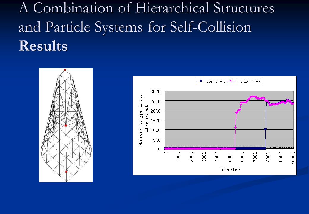
38. A Combination of Hierarchical Structures and Particle Systems for Self-Collision Results

40. A Combination of Hierarchical Structures and Particle Systems for Self-Collision Results Animation3.avi Animation3.avi

41. A Combination of Hierarchical Structures and Particle Systems for Self-Collision  Future work Improving the procedure of self-collision detection after particles detect a possibility Improving the procedure of self-collision detection after particles detect a possibility Investigating applicability for objects with changing topology Investigating applicability for objects with changing topology