1. Production

2. Objectives
To understand the concept of the short- run, diminishing returns and costs in the short run

3. The Short- run
a period of time where at least one factor of production is assumed to be in fixed supply i.e. it cannot be changed
Normally assumed that capital and physical land is fixed and that production can be altered through changing labour or input of raw materials

4. The Production Function
A mathematical expression which relates the quantity of factor inputs to the quantity of outputs that result.
Three measures of production / productivity
Total product = total output
Average product = the total output divided by the number of units of the variable factor of production employed (e.g. output per worker or output per unit of capital employed)
Marginal product = the change in total product when an additional unit of the variable factor of production is employed. For example marginal product would measure the change in output that comes from increasing the employment of labour by one person, or by adding one more machine to the production process in the short run

5. The Law of Diminishing Returns: A Simple Demonstration
Terry D. McCraney, Vincennes University
I use a simple example to explain the law of diminishing returns to students--sweeping the classroom floor. I usually start by stating the law as simply as possible. Then I tell the class that we have the job of sweeping the floor. All students agree that they are interchangeable when it comes to sweeping. They can all sweep and all can sweep equally well. I ask them how to measure our efficiency, if all sweep equally well. The general response is that we can measure efficiency in terms of time. Then I explain that we have four brooms and I will choose people to serve as sweepers. I choose the first sweeper and tell him it will take 60 minutes to do the job. The use of 60 minutes is for easy division. If you must, you can remind the students that the job was never done before so we have no idea how long it will take to complete the job. A second student is chosen and I ask how long it will take with two sweepers. The response is thirty minutes. Questions may be asked to explain the thirty minute time. After a third sweeper is added the time falls to twenty minutes. A fourth sweeper brings the time to fifteen minutes. Then I add a fifth sweeper and ask for the time. Twelve minutes will be given as the logical answer. Now I explain that twelve minutes is incorrect, and that it will take twenty-four minutes. I ask the students to explain why it took longer with five sweepers than with four. Most of the class will quickly point out that we only have four brooms. Then I restate the law of diminishing returns stressing that sweepers are inputs, brooms are the fixed factors, and the amount of time reflects marginal returns

6. Example- Law of diminishing returns
A firm has 4 machines (fixed factors) and increases it’s output by using more operators to work the machines
Production figures per week are in the following table…

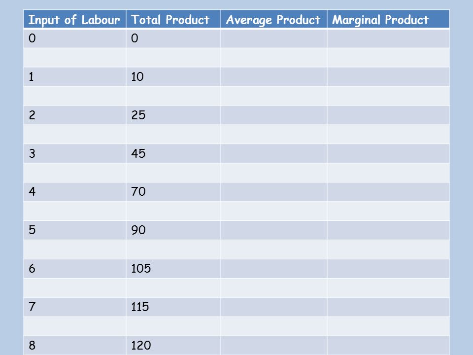
7. Input of Labour
Total Product
Average Product
Marginal Product 1 10 2 25 3 45 4 70 5 90 6
105 7
115 8
120

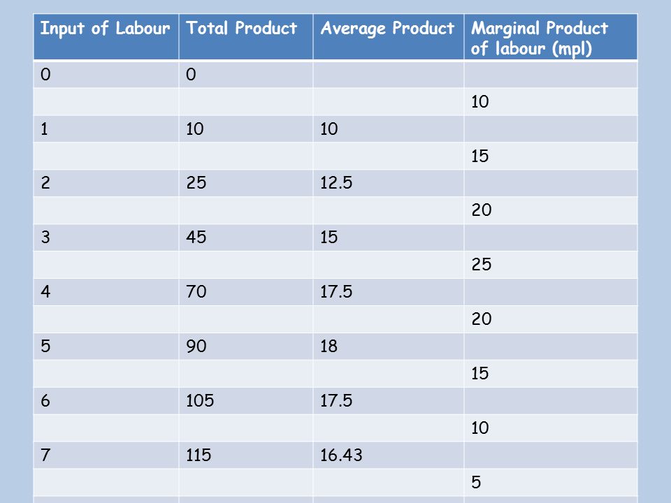
8. Input of Labour
Total Product
Average Product
Marginal Product of labour (mpl) 10 1 15 2 25
12.5 20 3 45 4 70
17.5 5 90 18 6
105 7
115
16.43 8
120

9. The Law of Diminishing Returns
In the short run, the law of diminishing returns states that
As more units of a variable input (i.e. labour or raw materials) is added to fixed amounts of land and capital, the change in total output will at first rise and then fall
In example
Diminishing returns to labour occurs when the mpl starts to fall.
This means that total output will still be rising – but increasing at a decreasing rate as more workers are employed.
Eventually a decline in marginal product leads to a fall in average product
As a result, the marginal productivity of each worker tends to fall – this is known as the principle of diminishing returns.   

10. Handout

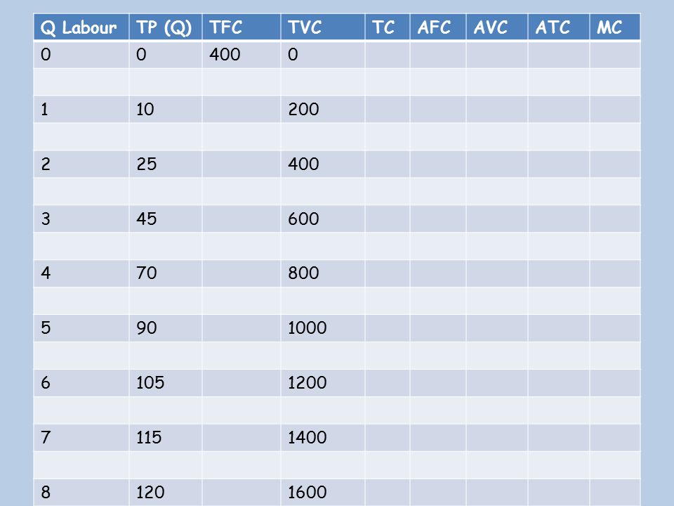
11. Short- run costs Fixed costs- do not vary with output
Variable Costs- vary directly with output
Total cost= fixed costs + variable costs
Average Cost= Total costs/ output
Marginal Cost= addition to total cost when one extra unit of output is produced

12. Q Labour
TP (Q)
TFC
TVC TC
AFC
AVC
ATC MC
400 1 10
200 2 25 3 45
600 4 70
800 5 90
1000 6
105
1200 7
115
1400 8
120
1600

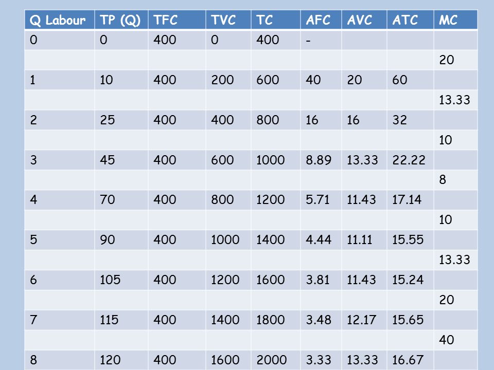
13. Q Labour
TP (Q)
TFC
TVC TC
AFC
AVC
ATC MC
400 - 20 1 10
200
600 40 60
13.33 2 25
800 16 32 3 45
1000
8.89
22.22 8 4 70
1200
5.71
11.43
17.14 5 90
1400
4.44
11.11
15.55 6
105
1600
3.81
15.24 7
115
1800
3.48
12.17
15.65
120
2000
3.33
16.67

14. On graph Paper
Plot the TC, TFC and TVC

15. Average Costs Costs per unit of output
Plot the AFC, AVC and ATC on a separate graph
Why are the AC curves shaped as they are?
Average Fixed Costs- Because TFC is constant AFC always falls as output increases
Average Variable Costs- Tends to fall as output rises (due to increasing returns to the variable factor as more are employed and more specialised methods are adopted) and then starts to rise again as output continues to increase, this is due to the concept of diminishing returns
Average cost (AC) (or average total cost (ATC)) = AFC + AVC and is therefore ‘U’ shaped because of the reasons above
Now plot the MC curve on this graph

16. Marginal Costs
MC tends to fall as output increases, and then starts to rise again as output continues to increase.
Explained by the concept of diminishing returns.

17. Relationship between AC, AVC and MC curve
The MC curve cuts the AVC and AC curve at their lowest points
AFC falls as output increases and, since it is the difference between AC and AVC, the vertical gap between AC and AVC gets smaller as output grows.

18. Illustrated…

19. AC
Output MC
AVC
Optimum Output MC= ATC

20. The MC and AC of Late Arrivals at Small Parties
Frederick S. Weaver, Hampshire College
How can the marginal cost curve start rising before the average cost curve does? Why does the marginal cost curve always intersect the average cost curve as its minimum point? These are simply arithmetic relationships, but they do confuse students and are sufficiently important to the theory of the firm that they warrant some special attention. An example that works for me is to ask students to imagine a small gathering of, say, ten people, and the average height of those at the party is 5'7". But some people are still arriving, and a latecomer who is 5'2" tall arrives at the party. What does this marginal guest do to the average height of those at the party (i.e., what direction does it change)? Another person, who is 5'3" arrives, and the average height of the roomful of revelers is pulled down a bit more. Yet another character drifts in, and her height is 5'6". The average height again declines (to 5'7"), as it has consistently even though the successive marginal changes have been getting larger. So as long as the increments are below the average, the average declines. Anyway, back to the party: when a person who is 5'7" joins the party, the average is unchanged, and when someone 5'8" tall finally manages to get there, the average height rises. So when a person of average height joints the festivities, the average does not change, but when someone above average height appears on the scene, the average height rises. Ergo, the marginal curve intersects the average curve at the average curve's minimum point.
Only directions of change rather than the particular numbers matter, but from experience, it pays to have a clear numerical example worked out before class. Initial confusion may facilitate understanding of some analytical issues, but this is not one of them!