1. 10
OUTPUT AND COSTS
CHAPTER

2. Objectives After studying this chapter, you will able to
Distinguish between the short run and the long run
Explain the relationship between a firm’s output and labor employed in the short run
Explain the relationship between a firm’s output and costs in the short run
Derive and explain a firm’s short-run cost curves
Explain the relationship between a firm’s output and costs in the long run
Derive and explain a firm’s long-run average cost curve

3. Decision Time Frames
The firm makes many decisions to achieve its main objective: profit maximization.
All decisions can be placed in two time frames:
The short run
The long run
The big picture
Stand back from the details of this chapter and be sure that your students learn two big ideas:
A firm’s production costs depend on the freedom to choose all inputs.
Long-run flexibility enables firms to produce at a lower cost than is possible in the short run when some inputs are fixed.
In the short run, with one or more fixed inputs, production costs vary with output in a predictable way because they are directly linked to input productivity.
Also, preview where we are heading. We want to be able to predict firm’s decisions.
To do so, we need to know about the influences on their costs and revenues.
Cost conditions are similar for all firms. That’s what we study here.
Revenue conditions depend on the market constraints. That’s what we study in the three chapters that follow.
Emphasize that what the student learns hear about cost is a vital prerequisite for understanding firms in perfect competition, monopoly, monopolistic competition, and oligopoly.

4. Decision Time Frames The Short Run
The short run is a time frame in which the quantity of one or more resources used in production is fixed.
For most firms, the capital, is fixed in the short run.
Other resources used by the firm (such as labor, raw materials, and energy) can be changed in the short run.
The Long Run
The long run is a time frame in which the quantities of all resources can be varied.

5. Short-Run Technology Constraint
To increase output in the short run, a firm must increase the amount of labor employed.
Three concepts describe the relationship between output and the quantity of labor employed:
Total product
Marginal product
Average product
Lots of definitions and terminology can cloud the primary message
Make good use of the glossary of productivity and cost terms provided in Table 10.2 (page 223) but don’t get mired down in reciting productivity and cost measure definitions!
Emphasize to the students that they must learn these definitions. But don’t spend a lot of class time on them.
Focus on why productivity measures and cost measures are vital for decision making.
Managers must frequently make quick decisions with little information. If managers have knowledge of a useful relationship between input measures (which are relatively easy to get) and production cost measures (which are much more difficult to get—especially marginal cost figures) they can use their understanding of this link to make inferences about how production costs will change when the firm’s output changes.

6. Short-Run Technology Constraint
Product Schedules
Total product is the total output produced in a given period.
The marginal product of labor is the change in total product that results from a one-unit increase in the quantity of labor employed, with all other inputs remaining the same.
The average product of labor is equal to total product divided by the quantity of labor employed.
Table 10.1 on page 215 shows a firm’s product schedules.

7. Short-Run Technology Constraint
Product Curves
total product, marginal product, and average product change as the quantity of labor employed changes.

8. Short-Run Technology Constraint
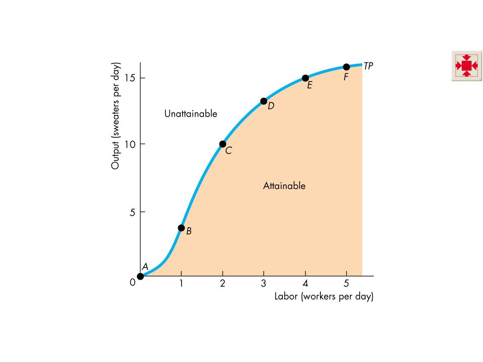
The Total Product Curve
Figure 10.1 shows a total product curve.
The total product curve shows how total product changes with the quantity of labor employed.

10. Short-Run Technology Constraint
The total product curve is similar to the PPF.
It separates attainable output levels from unattainable output levels in the short run.

12. Short-Run Technology Constraint
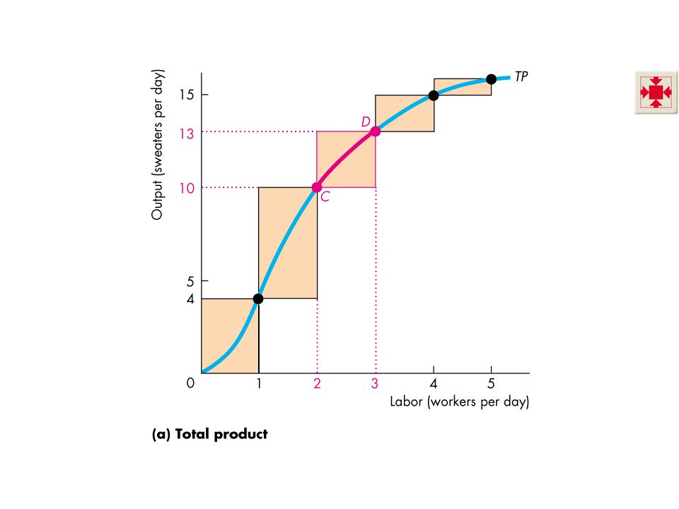
The Marginal Product Curve
Figure 10.2 shows the marginal product of labor curve and how the marginal product curve relates to the total product curve.
The first worker hired produces 4 units of output.

14. Short-Run Technology Constraint
The second worker hired produces 6 units of output and total product becomes 10 units.
The third worker hired produces 3 units of output and total product becomes 13 units.
And so on.

16. Short-Run Technology Constraint
The height of each bar measures the marginal product of labor.
For example, when labor increases from 2 to 3, total product increases from 10 to 13, so the marginal product of the third worker is 3 units of output.

18. Short-Run Technology Constraint
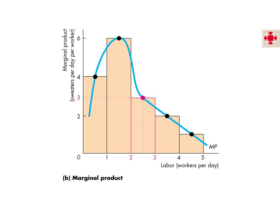
To make a graph of the marginal product of labor, we can stack the bars in the previous graph side by side.
The marginal product of labor curve passes through the mid-points of these bars.

20. Short-Run Technology Constraint
Almost all production processes are like the one shown here and have:
Initially increasing marginal returns
Eventually diminishing marginal returns

22. Short-Run Technology Constraint
Initially increasing marginal returns
When the marginal product of a worker exceeds the marginal product of the previous worker, the marginal product of labor increases and the firm experiences increasing marginal returns.

24. Short-Run Technology Constraint
Eventually diminishing marginal returns
When the marginal product of a worker is less than the marginal product of the previous worker, the marginal product of labor decreases and the firm experiences diminishing marginal returns.

26. Short-Run Technology Constraint
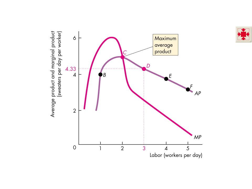
Average Product Curve
Figure 10.3 shows the average product curve and its relationship with the marginal product curve.
When marginal product exceeds average product, average product increases.
The marginal pulls (but cannot not push) the average
Don’t let the students fall into the trap of thinking that if the marginal measure rises (falls) with the level of an activity, then the average measure must also rise (fall). This is a sloppy statement of the relationship between marginal and average measures. Use the tried-and-true grade point average example used in the text. Explain that if their grade point average (GPA) is a 3.5, and their next marginal class grade is a C (2.0), followed by a B (3.0), this increasing marginal grade will not be pushing their GPA up at all. Conceptually, the students should understand that the marginal value can’t “push” the average measure higher when it is, itself, lower than the average measure. The marginal measure must be higher (lower) than the average value if the average value is to rise (fall) with the level of activity, thereby “pulling” the average from its position of either higher or lower than the average.

28. Short-Run Technology Constraint
When marginal product is below average product, average product decreases.
When marginal product equals average product, average product is at its maximum.

30. Short-Run Cost
To produce more output in the short run, the firm must employ more labor, which means that it must increase its costs.
We describe the way a firm’s costs change as total product changes by using three cost concepts and three types of cost curve:
Total cost
Marginal cost
Average cost
Explain the intuition behind each cost measure. For example, explain why the relationship between marginal product and marginal cost is worth understanding.
Point out that although separating fixed and variable components of cost help us understand why unit cost of production is U-shaped in the short run and why fixed costs don’t matter in a firm’s output decision.

31. Short-Run Cost TC = TFC + TVC Total Cost
A firm’s total cost (TC) is the cost of all resources used.
Total fixed cost (TFC) is the cost of the firm’s fixed inputs. Fixed costs do not change with output.
Total variable cost (TVC) is the cost of the firm’s variable inputs. Variable costs do change with output.
Total cost equals total fixed cost plus total variable cost. That is:
TC = TFC + TVC

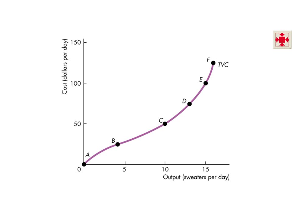
32. Short-Run Cost Figure 10.4 shows a firms total cost curves.
Total fixed cost is the same at each output level.
Total variable cost increases as output increases.
Total cost, which is the sum of TFC and TVC also increases as output increases.

34. Short-Run Cost
The total variable cost curve gets its shape from the total product curve.
Notice that the TP curve becomes steeper at low output levels and then less steep at high output levels.
Emphasize that the TP curve graph has labor on the x-axis and output on the y- axis, while the TVC curve has output on the x-axis and total variable cost on the y-axis. So, each graph has output on one of the axes.
In contrast, the TVC curve becomes less steep at low output levels and steeper at high output levels.

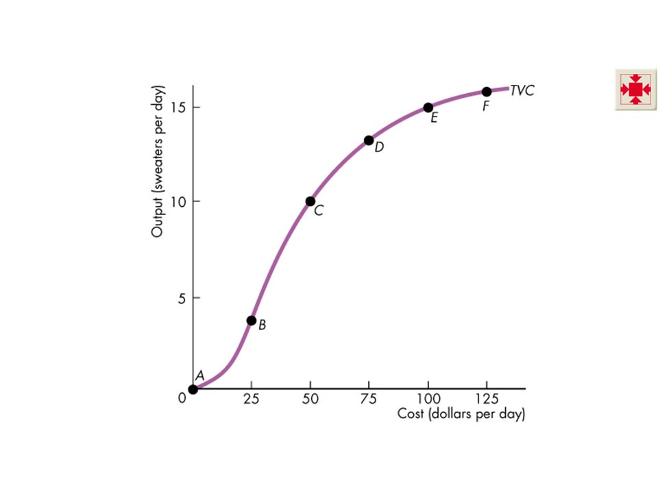
36. Short-Run Cost
To see the relationship between the TVC curve and the TP curve, lets look again at the TP curve.
But let us add a second x-axis to measure total variable cost.
1 worker costs $25; 2 workers cost $50: and so on, so the two x-axes line up.

38. Short-Run Cost
We can replace the quantity of labor on the x-axis with total variable cost.
When we do that, we must change the name of the curve. It is now the TVC curve.
But it is graphed with cost on the x-axis and output on the y-axis.

40. Short-Run Cost
Redraw the graph with cost on the y-axis and output on the x-axis, and you’ve got the TVC curve drawn the usual way.
Put the TFC curve back in the figure,
and add TFC to TVC, and you’ve got the TC curve.

42. Short-Run Cost Marginal Cost
Marginal cost (MC) is the increase in total cost that results from a one-unit increase in total product.
Over the output range with increasing marginal returns, marginal cost falls as output increases.
Over the output range with diminishing marginal returns, marginal cost rises as output increases.

43. Short-Run Cost ATC = AFC + AVC. Average Cost
Average cost measures can be derived from each of the total cost measures:
Average fixed cost (AFC) is total fixed cost per unit of output.
Average variable cost (AVC) is total variable cost per unit of output.
Average total cost (ATC) is total cost per unit of output.
ATC = AFC + AVC.

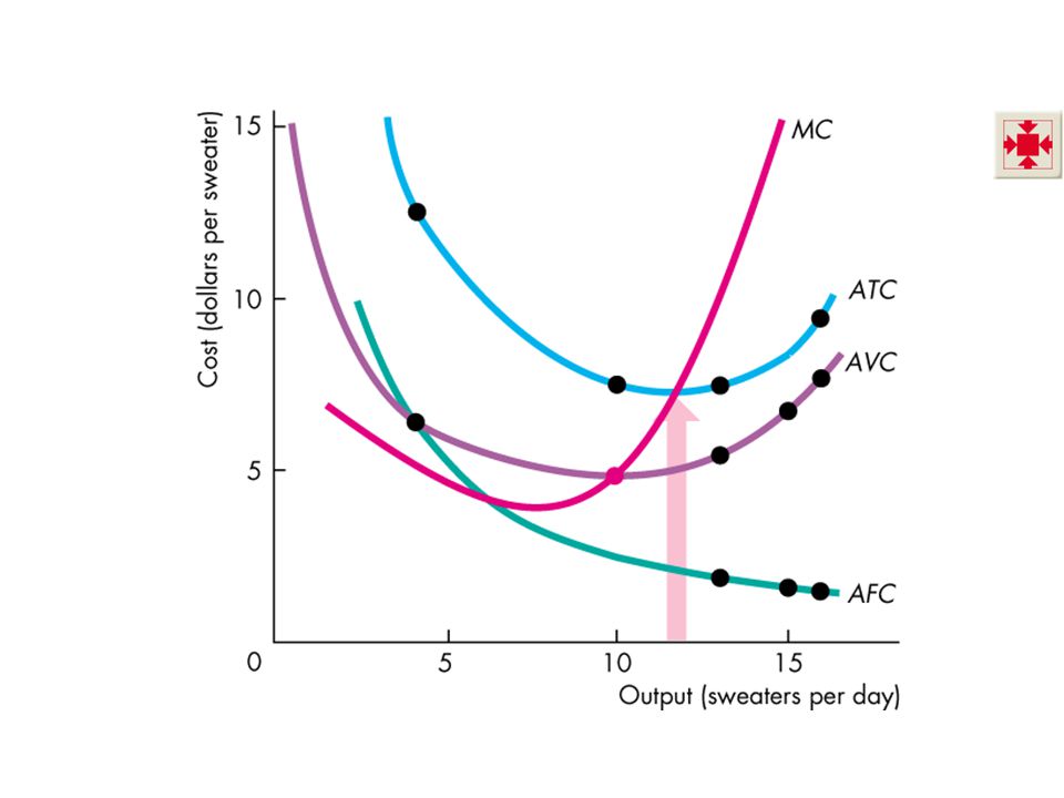
44. Short-Run Cost Figure 10.5 shows the MC, AFC, AVC, and ATC curves.
The AFC curve shows that average fixed cost falls as output increases.
The AVC curve is U-shaped. As output increases, average variable cost falls to a minimum and then increases.

46. Short-Run Cost The ATC curve is also U-shaped.
The MC curve is very special.
Where AVC is falling, MC is below AVC.
Where AVC is rising, MC is above AVC.
At the minimum AVC, MC equals AVC.

48. Short-Run Cost Similarly, where ATC is falling, MC is below ATC.
Where ATC is rising, MC is above ATC.
At the minimum ATC, MC equals ATC.

50. Short-Run Cost Cost Curves and Product Curves
The shapes of a firm’s cost curves are determined by the technology it uses:
MC is at its minimum at the same output level at which marginal product is at its maximum.
When marginal product is rising, marginal cost is falling.
AVC is at its minimum at the same output level at which average product is at its maximum.
When average product is rising, average variable cost is falling.

51. Short-Run Cost
Figure 10.6 shows these relationships.

53. Short-Run Cost Shifts in Cost Curves
The position of a firm’s cost curves depend on two factors:
Technology
Prices of productive resources

54. Long-Run Cost Short-Run Cost and Long-Run Cost
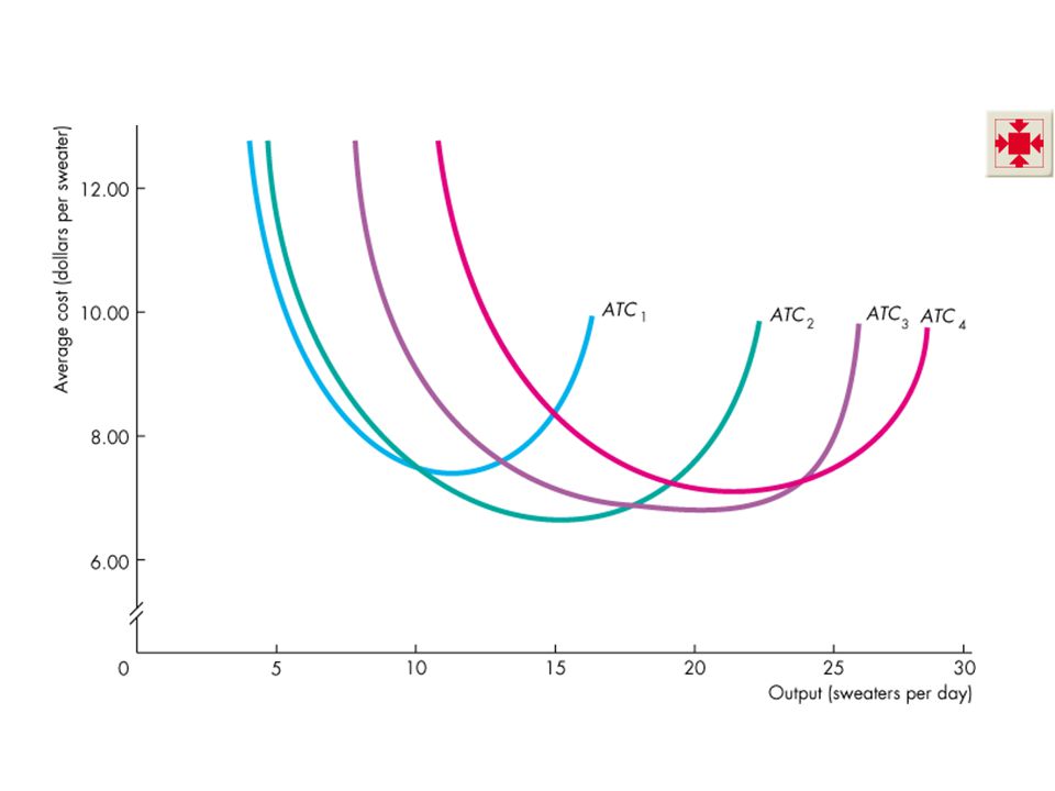
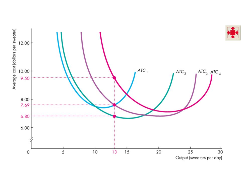
The average cost of producing a given output varies and depends on the firm’s plant size.
The larger the plant size, the greater is the output at which ATC is at a minimum.
Cindy has 4 different plant sizes: 1, 2, 3, or 4 knitting machines.
Each plant has a short-run ATC curve.
The firm can compare the ATC for each given output at different plant sizes.

55. Long-Run Cost
ATC1 is the ATC curve for a plant with 1 knitting machine.

57. Long-Run Cost
ATC2 is the ATC curve for a plant with 2 knitting machines.

59. Long-Run Cost
ATC3 is the ATC curve for a plant with 3 knitting machines.

61. Long-Run Cost
ATC4 is the ATC curve for a plant with 4 knitting machines.

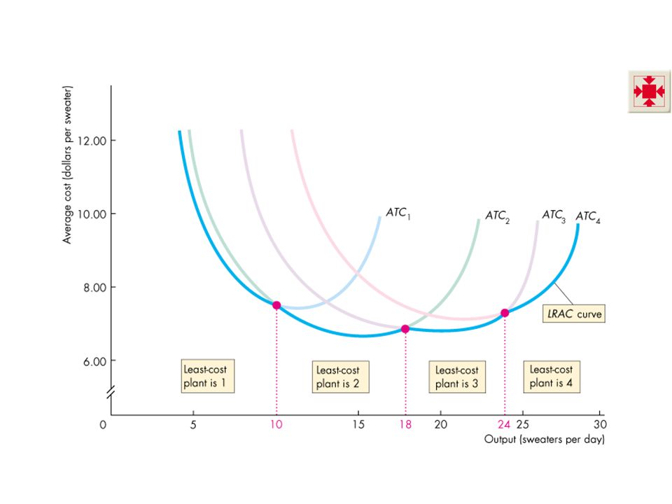
63. Long-Run Cost
The long-run average cost curve is made up from the lowest ATC for each output level.
So, we want to decide which plant has the lowest cost for producing each output level.
Let’s find the least cost way of producing a given output level.
Suppose that Cindy wants to produce 13 sweaters a day.

64. Long-Run Cost
13 sweaters a day cost $7.69 each on ATC1.

66. Long-Run Cost
13 sweaters a day cost $6.80 each on ATC2.

68. Long-Run Cost
13 sweaters a day cost $7.69 each on ATC3.

70. Long-Run Cost
13 sweaters a day cost $9.50 each on ATC4.

72. Long-Run Cost 13 sweaters a day cost $6.80 each on ATC2.
The least-cost way of producing 13 sweaters a day

74. Long-Run Cost Long-Run Average Cost Curve
The long-run average cost curve is the relationship between the lowest attainable average total cost and ouptut when both the plant size and labor are varied.
The long-run average cost curve is a planning curve that tells the firm the plant size that minimizes the cost of producing a given output range.

75. Long-Run Cost
Figure 10.8 illustrates the long-run average cost (LRAC) curve.

77. Long-Run Cost Economies and Diseconomies of Scale
Economies of scale: falling long-run average cost as output increases.
Diseconomies of scale: rising long-run average cost as output increases.
Constant returns to scale: constant long-run average cost as output increases.

78. Long-Run Cost
Figure 10.8 illustrates economies and diseconomies of scale.

80. Long-Run Cost
Minimum efficient scale(MES) is the smallest quantity of output at which the long-run average cost reaches its lowest level.
If the long-run average cost curve is U-shaped, the minimum point identifies the minimum efficient scale output level.

81. THE END