1. Summer Seminar Ruizhen Hu

2. Spectral Sampling of Manifolds (Siggraph Asia 2010) Accurate Multidimensional Poisson-Disk Sampling (TOG) Efficient Maximal Poisson-Disk Sampling Blue-Noise Point Sampling using Kernel Density Model Differential Domain Analysis for Non-uniform Sampling Sampling Noise & filtering Filtering Solid Gabor Noise Accelerating Spatially Varying Gaussian

3. Spectral Sampling of Manifolds A. Cengiz Öztireli Marc Alexa Markus Gross ETH Zürich TU Berlin ETH Zürich

4. Authors CENGİZ ÖZTİRELİ PhD Candidate Computer Graphics Laboratory ETH Zürich Research interests: Reconstruction, sampling and processing of surfaces, and sketch based modeling. Marc Alexa Professor Electrical Engineering & Computer Science TU Berlin Markus Gross Professor Department of Computer Science ETH Zürich Research interests: Computer graphics, image generation, geometric modeling, computer animation, and scientific visualization

5. Motivation Goal: finding optimal sampling conditions for a given surface representation Work: propose a new method to solve this problem based on spectral analysis of manifolds, kernel methods and matrix perturbation theory

6. Contributions Efficient, simple to implement, easy to control through intuitive parameters, feature sensitive Result in accurate reconstructions with kernel based approximation methods and high quality isotropic samplings A discrete spectral analysis of manifolds using results from kernel methods and matrix perturbation theory

7. Main Algorithm Input: a set of points lying near a manifold with normals + a kernel function definition = a continuous surface

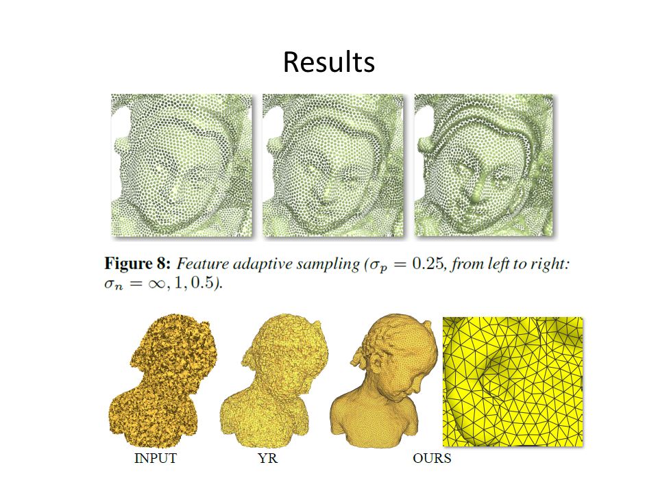
8. Algorithms for Sampling Subsampling: measuring the effect of a point on the manifold using the Laplace-Beltrami spectrum measures the contribution of a point to the manifold definition

9. Algorithms for Sampling Resampling: maximizing and equalizing s (x) for all points – use local operations and move points in a simple gradient ascent

10. Results

13. Conclusions New algorithms for the simplification and resampling of manifolds depending on a measure that restricts changes to the Laplace-Beltrami spectrum Limitations: the algorithms are greedy and thus not theoretically guaranteed to give the optimal sampling Future Directions: – texture on a surface – isotropic adaptive remeshing

14. Accurate Multi-Dimensional Poisson-Disk Sampling Manuel N. Gamito Steve Maddock Lightwork Design Ltd The University of Sheffield

15. Authors Manuel Noronha Gamito software engineer Lightwork Design Ltd Steve Maddock Senior Lecturer The University of Sheffield Research interests: character animation, specifically modelling and animating faces

16. Poisson-Disk Sampling Definition: – Each sample is placed with uniform probability density – No two samples are closer than, where is some chosen distribution radius – A distribution is maximal if no more samples can be inserted Poisson-Disk sampling is useful for: – Distributed ray tracing [Cook 1986; Hachisuka et al. 2008] – Object placement and texturing [Lagae and Dutré 2006; Cline et al. 2009] – Stippling and dithering [Deussen et al. 2000; Secord et al. 2002] – Global Illumination [Lehtinen et al. 2008]

17. Previous Methods Approximate Methods – Relax at least one of the sampling conditions Accurate Methods – Brute force Dart Throwing [Dippé and Wold 1985] – Assisted by a spatial data structure Voronoi diagram [Jones 2006] Scalloped sectors [Dunbar and Humphreys 2006] Uniform grid [Bridson 2007] Simplified subdivision tree and uniform grid [White et al. 2007]

18. Main Algorithm

19. Radius vs. Number of Samples A distribution can be specified by supplying either – The distribution radius r – The desired number of samples N When the number of samples is specified – The algorithm uses a radius r based on N and on the measured packing density of sample disks The packing density was obtained by averaging the packing densities measured from 100 distributions generated by our algorithm The number of samples of the resulting maximal distribution is approximately equal to the desired number N (error<5%)

20. Results Number of samples Sampling time Samples per second

21. Results

22. Conclusions A Poisson-Disk Sampling Algorithm that – Is statistically correct (see proof in paper) – Is efficient through the use of a subdivision tree – Works in any number of dimensions Subject to available physical memory – Generates maximal distributions – Allows approximate control over the number of samples – Can enforce periodic or wall boundary conditions on the boundaries of the domain

23. Future Work Make it multi-threaded – Distant parts of the domain can be sampled in parallel with different threads – Some synchronisation between threads is still required Generate non-uniform distributions – Have the distribution radius be a function of the position in the domain Work over irregular domains – Discard subdivided tree nodes that fall outside the domain

24. Efficient Maximal Poisson-Disk Sampling

25. Authors Mohamed S. Ebeida post-doctor Carnegie Mellon university Anjul Patney PhD Carnegie University of California, Davis Scott A. Mitchell Principal Member of Technical Staff Sandia National Laboratories Andrew Davidson PhD Carnegie University of California, Davis Patrick M. Knupp Distinguished Member Technical Staff Sandia National Laboratories John D. Owens Associate Professor Carnegie University of California, Davis

26. Work generating a uniform Poisson-disk sampling that is both maximal and unbiased over bounded non-convex domains

27. Motivation Maximal Poisson-disk sampling distributions: – Avoid aliasing – Have blue noise property Bias-free: – Crucial in fracture propagation simulations

28. Conditions Maximal : the sample disks overlap cover the whole domain leaving no room to insert an additional point Bias-free the likelihood of a sample being inside any subdomain is proportional to the area of the subdomain, provided the subdomain is completely outside all prior samples’ disks

29. Previous methods relax the unbiased or maximal conditions, or require potentially unbounded time or space Dart-throwing – unbiased but also not maximal Tile-based – biased and require relatively large storage.

30. Main Algorithm First phase: – an unbiased, near-maximal covering – voids: the part of a grid cell outside all circles Second phase: – completes the maximal covering – darts are thrown directly into the voids, maintaining the bias- free condition – A maximal distribution is achieved when the domain is completely covered, leaving no room for new points to be selected

31. Sequential Sampling 1.Generate a background grid; mark interior and boundary cells 2.Phase I. Throw darts into square cells; remove hit cells 3.Generate polygonal approximations to the remaining voids 4.Phase II. Throw darts into voids; update remaining areas

32. Algorithm through Phase I

33. Voids Polygonal approximations to arc-voids

34. Results

35. Implementation Performance

36. Conclusions An efficient algorithm for maximal Poisson-disk sampling in two-dimensions – the final result is provably maximal – the sampling is unbiased – it is O(n log n) in expected time – it is O(n) in deterministic memory required – not limited to convex domains – efficiently implemented in both sequential and parallel forms Future work: 3D maximal Poisson-disk sampling algorithm

37. Blue-Noise Point Sampling using Kernel Density Model Raanan Fattal Hebrew University of Jerusalem, Israel

38. Author Raanan Fattal Alon faculty member School of Computer Science and Engineering The Hebrew University of Jerusalem

39. Work A new approach for generating point sets with high-quality blue noise properties that formulates the problem using a statistical mechanics interacting particle model

40. Contributions present a new approach that formulates the problem using a statistical mechanics interacting particle model derive a highly efficient multi-scale sampling scheme for drawing random point distributions avoids the critical slowing down phenomena that plagues this type of models

41. Previous work Dart throwing – constrain a minimal distance between every pair of points Relaxation – follow a greedy strategy that maximizes this distance – two main shortcomings: teriminatin impreciseness : apparent blur

42. New Approach model the target density as a sum of nonnegative radially- symmetric kernels The j-th kernel centered around the point x j:

43. New Approach The error of this approximation Minimizing E, with respect to the kernel centers – equivalent to the one obtained by converged Lloyd’s iterations – has the ability to achieve spectral enhancement We unify error minimization and randomness by defining a statistical mechanics particle model using E

44. New Approach Assigning each configuration a probability density according to the following Boltzmann- Gibbs distribution:

45. Drawing samples Markov-chain Monte Carlo(MCMC) Gibbs sampler Langevin method Metropolis-Hastings(MH) test

46. Critical slowing down

47. Multi-scale sampling

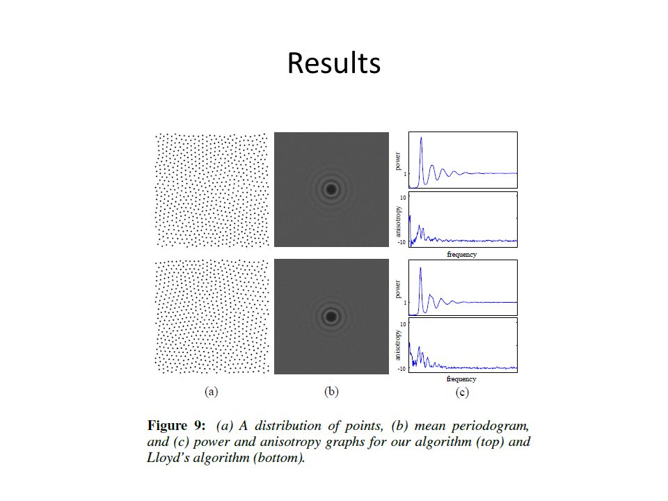
48. Results

50. Differential Domain Analysis for Non-uniform Sampling Li-Yi Wei Rui Wang Microsoft Research University of Massachusetts Amherst

51. Authors Li-Yi Wei Researcher Microsoft Research Rui Wang Assistant Professor Department of Computer Science University of Massachusetts

52. Work new methods for analyzing non-uniform sample distributions

53. Previous work Two common methodologies exist for evaluating the quality of samples – spatial uniformity: discrepancy & relative radius – Power spectrum analysis, including radial mean and anisotropy However, existing methods are primarily designed for uniform Euclidean domains and can not be easily extended to general non-uniform scenarios, such as – adaptive – anisotropic – non-Euclidean domains

54. Contributions A reformulation of standard Fourier spectrum analysis into a form that depends on sample location differentials A generalization of this basic formulation, including different distance transformations for various domains, and range selection for better control of quality and speed Applications in spectral and spatial analysis for non-uniform sample distributions

55. Core idea Fourier power spectrum – Fourier transform: – power spectrum: Differential representation:

56. Core idea Integral form: General kernel: – Range selection (for computational reasons): Where is a local distance measure of s’ with respect to the local frame centered at s. In uniform Euclidean domains,

57. Core idea Non-uniform domain ： Where is a differential domain transformation function that locally warps each d from a non-uniform to a (hypothetical) uniform

58. Kernel selection a cos kernel may amplify some information while obscure others A Gaussian kernel, in contrast, displays the main peak clearly without undulations. it can manifest the distribution properties more clearly, e.g. more apparent characteristic structures

59. Spectral Analysis Exact – Isotropic Euclidean domain – Anisotropic Euclidean domain Range selection Radial measures – We can compute the circular average and variance of p(d) – The former gives the radial mean, indicating the overall distance-based property of p(d) – The latter gives the anisotropy, which reveals if there is any directional bias/structure in the distribution

60. Comparisons How our method relates and compares to traditional Fourier spectrum analysis?

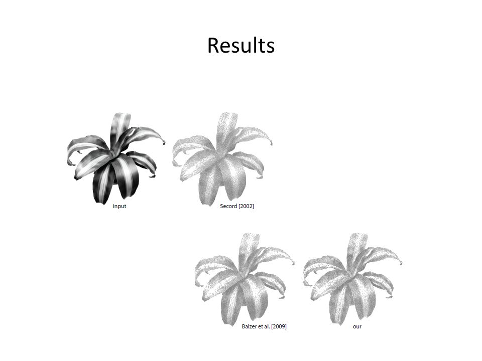
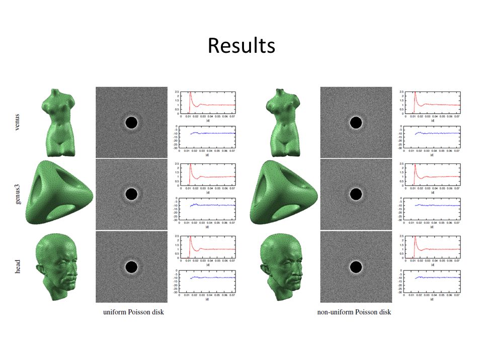
61. Results

63. Filtering Solid Gabor Noise Ares Lagae George Drettakis Katholieke Universiteit Leuven REVES/INRIA Sophia-Antipolis

64. Authors Ares Lagae Postdoctoral Fellow Computer Graphics Research Group Katholieke Universiteit Leuven George Drettakis Group Leader REVES/Inria Sophia-Antipolis

65. Work we show that a slicing approach is required to preserve continuity across sharp edges, and we present a new noise function that supports anisotropic filtering of sliced solid noise

66. Filtering Filtering the noise on the surface using frequency clamping works better if the power spectrum of the noise on the surface is bandpass. The Fourier Slice Theorem: projecting in the spatial domain corresponds to slicing in the frequency domain, and vice versa

67. Previous works Perlin noise[Perlin 1985]: – use slicing and frequency clamping – Filtering introduces an aliasing vs. detail loss trade-off since the power spectrum of Perlin noise is not band-pass Wavelet noise [Cook and DeRose 2005]: – use projection and frequency clamping – Even though the power spectrum of the noise on the surface is band-pass, filtering does not fully solve the aliasing vs. detail loss trade-off Gabor noise [Lagae et al. 2009]: – use projection and a filtering approach specific to Gabor noise – This results in high-quality anisotropic filtering, however, introduces discontinuities at sharp edges

68. New noise solid random-phase Gabor noise: – use slice (preserves continuity at sharp edges) – Since filtering is inherently a 2D operation, we have to explicitly model the slicing of the 3D Gabor kernels to be able to filter the resulting 2D Gabor kernels. This requires the introduction of a new Gabor kernel, the phase-augmented Gabor kernel a new Gabor noise, random-phase Gabor noise

69. Slicing Solid Gabor Noise The Gabor kernel of Lagae et al. [2009] is not closed under slicing:

70. Phase-augmented Gabor kernel The phase-augmented Gabor kernel is closed under slicing: solid random-phase Gabor noise (also closed under slicing):

71. Slicing Random-Phase Gabor Noise solid random-phase Gabor noise is also closed under slicing the statistical properties of a sliced solid random-phase Gabor noise are obtained using the analytical expressions for the statistical properties of a 2D random-phase Gabor noise

73. Filtering Sliced Solid Gabor Noise

74. Conclusion A new procedural noise function, random-phase Gabor noise, that supports – continuity across sharp edges – high-quality anisotropic filtering – Anisotropy Future work: – exploring volumetric filtering of solid Gabor noise – further exploring anisotropy in the context of solid noise – designing user interfaces for interacting with anisotropic solid noise

75. Results

77. Accelerating Spatially Varying Gaussian Filters Jongmin Baek David E. Jacobs Stanford University

78. Jongmin Baek Ph.D. student Stanford University David E. Jacobs PhD candidate Stanford University Authors

79. Motivation Input Gaussian Filter Spatially Varying Gaussian Filter

80. 1) Accelerating Spatially Varying Gaussian Filters 2) Accelerating Spatially Varying Gaussian Filters 3) Accelerating Spatially Varying Gaussian Filters 4) Applications Roadmap

81. Gaussian Filters Position Value

82. Gaussian Filters Each output value …

83. Gaussian Filters … is a weighted sum of input values …

84. Gaussian Filters … whose weight is a Gaussian …

85. Gaussian Filters … in the space of the associated positions.

86. Gaussian Blur Gaussian Filters: Uses

87. Bilateral Filter Gaussian Filters: Uses

88. Non-local Means Filter Gaussian Filters: Uses

89. Applications  Denoising images and meshes  Data fusion and upsampling  Abstraction / Stylization  Tone-mapping ... Gaussian Filters: Summary Previous work on fast Gaussian Filters  Bilateral Grid (Chen, Paris, Durand; 2007)  Gaussian KD-Tree (Adams et al.; 2009)  Permutohedral Lattice (Adams, Baek, Davis; 2010)

90. Summary of Previous Implementations:  A separable blur flanked by resampling operations.  Exploit the separability of the Gaussian kernel. Gaussian Filters: Implementations

91. Spatially Varying Gaussian Filters Spatially varying covariance matrix Spatially Invariant

92. Trilateral Filter (Choudhury and Tumblin, 2003)  Tilt the kernel of a bilateral filter along the image gradient.  “Piecewise linear” instead of “Piecewise constant” model. Spatial Variance in Previous Work

93. Spatially Varying Gaussian Filters: Tradeoff Benefits:  Can adapt the kernel spatially.  Better filtering performance. Cost:  No longer separable.  No existing acceleration schemes. Input Bilateral-filtered Trilateral-filtered

94. Problem:  Spatially varying (thus non-separable) Gaussian filter Existing Tool:  Fast algorithms for spatially invariant Gaussian filters Solution:  Re-formulate the problem to fit the tool.  Need to obey the “piecewise-constant” assumption Acceleration

95. Naïve Approach (Toy Example) I LOST THE GAME Input Signal Desired Kernel 111234 filtered w/ 1 filtered w/ 2 filtered w/ 3 filtered w/ 4 111 2 3 Output Signal 4

96. In practice, the # of kernels can be very large. Challenge #1 Pixel Location x Desired Kernel K(x) Range of Kernels needed

97. Sample a few kernels and interpolate. Solution #1 Desired Kernel K(x) Sampled kernels Interpolate result! Pixel Location x K1K1 K2K2 K3K3

98. Interpolation needs an extra assumption to work:  The covariance matrix Ʃ i is either piecewise-constant, or smoothly varying.  Kernel is spatially varying, but locally spatially invariant. Assumptions

99. Runtime scales with the # of sampled kernels. Challenge #2 Desired Kernel K(x) Filter only some regions of the image with each kernel. (“support”) Pixel Location x Sampled kernels K1K1 K2K2 K3K3

100. In this example, x needs to be in the support of K 1 & K 2. Defining the Support Desired Kernel K(x) Pixel Location x K1K1 K2K2 K3K3

101. Dilating the Support Desired Kernel K(x) Pixel Location x K1K1 K2K2 K3K3

102. Algorithm 1) Identify kernels to sample. 2) For each kernel, compute the support needed. 3) Dilate each support. 4) Filter each dilated support with its kernel. 5) Interpolate from the filtered results.

103. Algorithm 1) Identify kernels to sample. 2) For each kernel, compute the support needed. 3) Dilate each support. 4) Filter each dilated support with its kernel. 5) Interpolate from the filtered results. K1K1 K2K2 K3K3

104. Algorithm 1) Identify kernels to sample. 2) For each kernel, compute the support needed. 3) Dilate each support. 4) Filter each dilated support with its kernel. 5) Interpolate from the filtered results. K1K1 K2K2 K3K3

105. Algorithm 1) Identify kernels to sample. 2) For each kernel, compute the support needed. 3) Dilate each support. 4) Filter each dilated support with its kernel. 5) Interpolate from the filtered results. K1K1 K2K2 K3K3

106. Algorithm 1) Identify kernels to sample. 2) For each kernel, compute the support needed. 3) Dilate each support. 4) Filter each dilated support with its kernel. 5) Interpolate from the filtered results. K1K1 K2K2 K3K3

107. Algorithm 1) Identify kernels to sample. 2) For each kernel, compute the support needed. 3) Dilate each support. 4) Filter each dilated support with its kernel. 5) Interpolate from the filtered results. K1K1 K2K2 K3K3

108. Applications  HDR Tone-mapping  Joint Range Data Upsampling

109. Application #1: HDR Tone-mapping Input HDR Detail Base Filter Output Attenuate

110. Tone-mapping Example Bilateral Filter Kernel Sampling

111. Application #2: Joint Range Data Upsampling Range Finder Data  Sparse  Unstructured  Noisy Scene Image Output Filter

112. Synthetic Example Scene Image Ground Truth Depth

113. Synthetic Example Scene ImageSimulated Sensor Data

114. Synthetic Example : Result Kernel Sampling Bilateral Filter

115. Synthetic Example : Relative Error Bilateral Filter Kernel Sampling 2.41% Mean Relative Error0.95% Mean Relative Error

116. Real-World Example Scene Image Range Finder Data *Dataset courtesy of Jennifer Dolson, Stanford University

117. Real-World Example: Result Input Bilateral Naive Kernel Sampling

118. Performance Kernel Sampling Choudhury and Tumblin (2003) Naïve Tonemap1 5.10 s41.54 s312.70 s Tonemap2 6.30 s88.08 s528.99 s Kernel Sampling (No segmentation) Depth1 3.71 s57.90 s Depth2 9.18 s131.68 s

119. 1.A generalization of Gaussian filters Spatially varying kernels Lose the piecewise-constant assumption. 2.Acceleration via Kernel Sampling Filter only necessary pixels (and their support) and interpolate. 3.Applications Conclusion