1. When advection destroys balance, vertical circulations arise COMET-MSC Winter Weather Course 29 Nov. - 10 Dec. 2004 ppt started from one by James T. Moore Saint Louis University Cooperative Institute for Precipitation Systems Brian Mapes

2. Quasi-Geostrophic Theory It provides a framework to understand the evolution of balanced three-dimensional velocity fields. It reveals how the dual requirements of hydrostatic and geostrophic balance (encapsulated as thermal wind balance) constrain atmospheric motions. It helps us to understand how the balanced, geostrophic mass and momentum fields interact on the synoptic scale to create vertical circulations which result in sensible weather.

3. Stable balanced dynamics Deviations from balance lead to force imbalances that drive ageostrophic and vertical motions which adjust the state back toward balance. Consider hydrostatic, geostrophic as simplest case of balances. Houze chapter 11 - use Boussinesq, hydrostatic equation set as we did for gravity waves. Introduce pseudoheight Assume wind is mostly geostrophic u g, v g Note: f-plane approximation means  V g =0

4. Balance in atmospheric dynamics 1.The vertical equation of motion: imbalance between the 2 terms on the RHS results in small vertical motions that restore balance - unless the state is gravitationally unstable 2.The horizontal equation of motion: imbalance between the major terms on the RHS leads to small ageostrophic motions that restore balance - unless the state is inertially unstable 3.Between lies symmetric instability. Like gravitional instability, it has moist (potential, conditional) cousins. For now, STABLE CASE

5. Old school: Quasi-Geostrophic Omega Equation (vorticity-oriented form) A B C Term A: three-dimensional Laplacian of omega Term B: vertical variation of the geostrophic advection of the absolute geostrophic vorticity Term C: Laplacian of the geostrophic advection of thickness

6. Problems with the Traditional Form of Q-G Diagnostic Omega Equation The two forcing functions are NOT independent of each other The two forcing functions often oppose one another (e.g., PVA and cold air advection – who wins?) You need more than one level of information to estimate differential geostrophic vorticity advection You cannot estimate the Laplacian of the geostrophic thickness advection by eye! The forcing functions depend upon the reference frame within which they are measured (i.e., the forcing functions are NOT Galilean invariant)

7. PV view of how maintenance of balance requires vertical motions

8. cyclonic  (Trof) Thermal wind balance prevails: There is a Z trough (trof) for geostrophic balance, with a cold core beneath it, supporting it hypsometrically (in hydrostatic balance).

9. cyclonic (Trof) Unsheared advection of T, u, v, vort, PV: no problem, whole structure moves

10. Sheared advection breaks thermal wind balance cyclonic  (Trof)

11. Sheared advection breaks thermal wind balance Z Trof (hypsometric)

12. Sheared advection breaks thermal wind balance Z Trof (hypsometric)

13. The PV view of balanced circulation: (Rob Rogers’s fig) Long-lived Great Plains MCVHurricane Andrew after landfall Potential temperature and potential vorticity cross sections

14. Q-vector Form of the Q-G Diagnostic Omega Equation Alternate approach developed by Hoskins et al. (1978, Q. J.) – manipulated the equations so forcing is 1 term, not 2:

15. Q-vector Form of the Q-G Diagnostic Omega Equation Treat Laplacian as a “sign flip” Then, If -2 Q > 0 (convergence of Q) then  < 0 (upward vertical motion) If -2 Q 0 (downward vertical motion) The Q vector points along the ageostrophic wind in the lower branch of the secondary circulation Q vectors point toward the rising motion and are proportional to the strength of the horizontal ageostrophic wind

16. Advantages of Using Q Vectors You only need one isobaric level to compute the total forcing (although layers are probably better to use) Only one forcing term, so no cancellation between terms Plotting Q vectors indicates where the forcing for vertical motion is located and they are a good approximation for the ageostrophic wind The forcing function is not dependent on the reference frame (I.e., it is Galilean invariant Plotting Q vectors and isentropes can indicate regions of Q-G frontogenesis/frontolysis No term is neglected (as in the Trenberth method which neglects the deformation term)

17. Interpreting Q Vectors Setting aside the coefficients, Expanding Q and assuming adiabatic conditions yields the following expression for Q:

18. Interpretation of Q x coldwarm  ugug coldwarm Geostrophic stretching deformation weakens   cold warm Geostrophic shearing deformation turns  vgvg  cold warm toto to+tto+t

19. Interpretation of Q y coldwarm  ugug cold warm Geostrophic shearing deformation turns   cold warm Geostrophic stretching deformation strengthens  vgvg  cold warm toto to+tto+t

20. Keyser et al. (1992, MWR) derived a form of the Q vector in “natural” coordinates where one component is oriented parallel to isotherms and another component is oriented normal to the isotherms. In this form one component (Q s ) has the two shearing deformation terms, expressing rotation of isotherms, that normally show up in Q x and Q y. Meanwhile, the other component (Q n ) has the two stretching deformation terms expressing the contraction or expansion of isotherms. We will see that this novel form of the Q vector has distinct advantages, in terms of interpretation. An Alternative form of Q in “natural” coordinates

21. Defining the Orientation of Q s and Q n with Respect to  Martin (1999, MWR) Q s is the component of Q associated with rotating the thermal gradient. Q n is the component of Q associated with changing the magnitude of the thermal gradient.   -1  +1  +2  QsQs QnQn Q cold warm s n Keyser et al. (1992, MWR)

22. Defining Q n and Interpreting What It Means

23. Defining Q n and Interpreting What It Means (cont.)   +1  +2  v g /  y < 0; therefore Q n <0; Q n points from cold to warm air; confluence (diffluence) in wind field implies frontogenesis (frontolysis) QnQn  Couplets of div Q n : Tend to line up across the isotherms Show the ageostrophic response to the geostrophically-forced packing/unpacking of the isotherms Often exhibit narrow banded structures typical of the “frontal” scale Give an indication of how “active” a front might be

24. Interpreting Q vectors: Q n Advection by geostrophic stretching deformation acts to change the magnitude of the thermal gradient vector, . But the same geostrophic advection changes the wind shear in the direction OPPOSITE to that needed to restore balance. This is why the forcing for ageostrophic secondary circ is -2x( .Q)! cold Low level wind: pure geostrophic deformation (noting .V g = 0), here acting to weaken dT/dx. warm Thermal wind Upper level wind: add thermal wind to low level wind. v component is positive and decreases to north, so advection is acting to increase upper-level v.

25. Defining Q s and Interpreting What It Means

26. Defining Q s and Interpreting What It Means (cont.)   +1  +2   v g /  x > 0; therefore Q s > 0. Q s has cold air is to its left, causes cyclonic rotation of the vector . Thermal wind balance thus requires v to increase aloft, but geostrophic advection acts to decrease v aloft. QsQs QsQs Thermal wind Upper wind Couplets of div Q s : Tend to line up along the isotherms Show the ageostrophic response to the geostrophically-forced turning of the isotherms Tend to be oriented upstream and downstream of troughs Are associated with the synoptic wave scale of ascent and descent

27. Estimating Q vectors Sanders and Hoskins (1990, WAF) derived a form of the Q vector which could be used when looking at weather maps to qualitatively estimate its direction and magnitude: Where the x axis is defined to be along the isotherms (with cold air to the left) and y is normal to x and to the left. Thus, Q is large when the temperature gradient is strong and when the geostrophic shear along the isotherms is strong. To estimate the direction of Q just use vector subtraction to compute the derivative of V g along the isotherms, then rotate the vector by 90° in the clockwise direction. Example:

28. AB AB Holton (1992) A - B = Q A - B = Q Jet Entrance Region Col Region 90 deg Q vectors This is mainly the cross-front, n component Q n

29. Q vectors in a setting where warm air rises Q n vectors Direct Thermal Circulation Confluent Flow Holton, 1992 cold warm

30. V ageo North South V ageo Thermally Indirect Circulation Q Jet Exit Region Q vectors in a setting where COLD air rises

31. Holton (1992) Idealized pattern of sea-level isobars (solid) and isotherms (dashed) for a train of cyclones and anticyclones. Heavy bold arrows are Q vectors. This is mostly the along-front or s component Q s.

32. Layer-Mean Q s for 850-500 hPa 12 UTC 25 Feb 1993 Vertical motion associated with the 500 hPa short wave

33. Layer-Mean Q n for 850-500 hPa 12 UTC 25 Feb 1993 Vertical motion associated with the warm front

34. Summary of Q-G Theory and the Use of Q vectors Q-vector form of the omega equation provides a complete picture of Q-G forcing of vertical motion Factor of 2 times the Q-vector describes how advection by geostrophic wind conspires to destroy thermal wind balance with double effectiveness, by opposite effects on the thermal gradient and wind shear. Houze (11.10) Houze (11.12) Houze (11.13)

35. Summary of Q-G Theory and the Use of Q vectors Q-vector form of the omega equation provides a complete picture of Q-G forcing of vertical motion Factor of 2 times the Q-vector describes how advection by geostrophic wind conspires to destroy thermal wind balance with double effectiveness, by opposite effects on the thermal gradient and wind shear. Q-vector forcing creates an ageostrophic response in an attempt to restore thermal wind balance. This too has double effectiveness: The Coriolis force acting on the sheared ageostrophic wind adjusts the vertical shear of geostrophic wind, while the vertical motion branch of the circulation adjusts T (thickness) gradients. Houze (11.19-11.20) u a across 2D front

36. Summary of Q-G Theory and the Use of Q vectors (cont.) Static stability (incl. moist effects - condensation) modulates the amount of vertical motion resulting from a given Q-G forcing: balance requires a certain density gradient, not a vertical motion per se. If the atmosphere is neaer neutral to moist ascent, a large amount of vertical motion (and rainfall) may occur. Turning of isotherms is related to the along-isotherm Q s component of the Q-vector – resulting in cyclone-scale vertical motion patterns along the isotherms. Geostrophic frontogenesis/frontolysis Q n results in banded vertical motion features in the cross-frontal direction (where scales are typically smaller).

38. Semi-geostrophic extension to QG theory Allow advection of b and v by an ageostrophic horizontal wind u a in cross-front (x) direction only (following Houze section 11.2.2). An elegant trick: define Using the fact that Dv g /Dt = -fu a, the total derivative in X space becomes analogous to D g /Dt:

39. Semi-geostrophic extension to QG theory (cont) More elegant trickery: Defining the geostrophic PV (Houze 11.50) One can get the streamfunction equation (11.60) Comparing the QG case (11.20) PV plays the role of a static stability in this system.

40. Another form (from notes of R. Johnson, CSU) is met (translation: PV must be positive, so that the system is symmetrically stable)

41. Frontogenesis (definition)  The 2-D scalar frontogenesis function (F ): F > 0 frontogenesis, F < 0 frontolysis (S. Petterssen 1936)  F: generalization of the quasi-geostrophic version, the Q-vector  Can also include diabatic heating gradients, etc. Q g

43. Frontogenesis and Symmetric Instability

44. Symmetric instabilities, contributing to banded precipitation, often north and east of midlatitude cyclones

45. Mesoscale Instabilities and Processes Which Can Result in Enhanced Precipitation Conditional Instability Convective Instability Inertial Instability Potential Symmetric Instability Conditional Symmetric Instability Weak Symmetric Stability Convective-Symmetric Instability Frontogenesis

46. Balance in atmospheric dynamics 1.The vertical equation of motion: imbalance between the 2 terms on the RHS results in small vertical motions that restore balance - unless the state is gravitationally unstable 2.The horizontal equation of motion: imbalance between the major terms on the RHS leads to small ageostrophic motions that restore balance - unless the state is inertially unstable 3.Between lies symmetric instability. Like gravitional instability, it has moist (potential, conditional) cousins. For now, STABLE CASE

47. Schultz et al. 1999 MWR

48. Instabilities: nomenclature Schultz et al. MWR 1999 “The intricacies of instabilities”

49. Conditional Instability Conditional Instability is diagnosed through an examination of lapse rates of temperature or saturated equivalent potential temperature (  es ): (a)  m <  <  d ; where  = -dT/dz OR, equivalently (b)dh s /dz < 0; where h s = saturated moist static energy A saturated parcel will ascent/descend along moist adiabats and undergo free convection

50. Dryish aloft Very Dry aloft Neutral “Potentially” Unstable If ENTIRE layer is lifted ALL THE WAY TO SATURATION (this might be a looong way for very dry air), will it overturn? Dry adiabats are thin solid lines, saturation adiabats are dash-dot lines. Hess (1959) Potential Instability LCLs In green Absolutely unstable lapse rate

51. Inertial Instability Inertial instability is the horizontal analog to gravitational instability; i.e., if a parcel is displaced horizontally from its geostrophically balanced base state, will it return to its original position or will it accelerate further from that position? Inertially unstable regions are diagnosed where:  g + f < 0 (NH); absolute geostrophic vorticity anticyclonic OR  M g /  x < 0; absolute geostrophic momentum M g = v g + fx decreases with distance from the rotation axis Equatorward of a westerly jet where the anticyclonic shear is large In sub-synoptic ridges where the anticyclonic curvature is large

52. Typical Regions Where MCS Tend to Form with Respect to the Upper-Level Flow Blanchard, Cotton, and Brown, 1998 (MWR)

53. Conditional Symmetric Instability: Cross section of  es and M g taken normal to the 850-300 mb thickness contours  es M g +1  es + 1  es -1 MgMg M g -1 s Note: isentropes of  es are sloped more vertical than lines of absolute geostropic momentum, M g. Vert. stable Horiz. stable Symm.unstable

54. Conditional Symmetric Instability in the Presence of Synoptic Scale Lift – Slantwise Ascent and Descent Multiple Bands with Slantwise Ascent

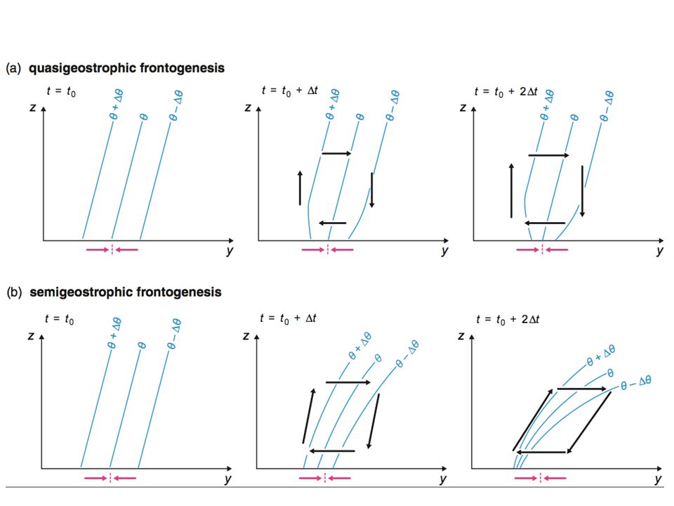
55. Frontogenesis and varying Symmetric Stability Emanuel (1985, JAS) has shown that in the presence of weak symmetric stability (simulating condensation) in the rising branch, the ageostrophic circulations in response to frontogenesis are changed. The upward branch becomes contracted and becomes stronger. The strong updraft is located ahead of the region of maximum geostrophic frontogenetical forcing. The distance between the front and the updraft is typically on the order of 50-200 km On the cold side of the frontogenetical forcing stability is greater and and the downward motion is broader and weaker than the updraft.

56. Frontal secondary circulation - constant stability Frontal secondary circ - with condensation on ascent Emanuel (1985, JAS)

57. Schematic of Convective-Symmetric Instability Circulation Blanchard, Cotton, and Brown, 1998 (MWR)

58. Convective-Symmetric Instability Multiple Erect Towers with Slantwise Descent

59. Sanders and Bosart, 1985: Mesoscale Structure in the Megalopolitan Snowstorm of 11-12 February 1983. J. Atmos. Sci., 42, 1050-1061.

60. As gravitational or symmetric stability decreases, the horizontal scale (width) of a precipitation band decreases while the intensity (reflectivity) of the band increases. Multiple bands become established in an unstable regime. Thus, it is very important to look for CSI and convectively unstable areas aloft besides just frontogenesis.

61. Frontogenesis and Symmetric Instability

62. NW SE NW-SE cross-section shown on next slide. A Conceptual Model: Plan View of Key Processes Often found in the vicinity of an extratropical cyclone warm front, ahead of a long- wave trough in a region of strong, moist, mid-tropospheric southwesterly flow

63. Dry Air  es Convectively Unstable Shaded area = CSI CSI Arrows = Ascent zone F = Frontogenesis zone Heavy snow area A Conceptual Model: Cross-Sectional View of Key Processes CSI may be a precursor to elevated CI, as the vertical circulation associated with CSI may overturn  e surfaces with time creating convectively unstable zones aloft

64. Nolan-Moore Conceptual Model Many heavy precipitation events display different types of mesoscale instabilities including: –Convective Instability (CI;  e decreasing with height) –Conditional Symmetric Instability (CSI; lines of  es are more vertical than lines of constant absolute geostrophic momentum or M g ) –Weak Symmetric Stability (WSS; lines of  es are nearly parallel to lines of constant absolute geostrophic momentum or M g )

65. Spectrum of Mesoscale Instabilities

66. Nolan-Moore Conceptual Model These mesoscale instabilities tend to develop from north to south in the presence of strong uni-directional wind shear (typically from the SW) CI tends to be in the warmer air to the south of the cyclone while CSI and WSS tend to develop further north in the presence of a cold, stable boundary layer. It is not unusual to see CI move north and become elevated, producing thundersnow.

67. Nolan-Moore Conceptual Model CSI may be a precursor to elevated CI, as the vertical circulation associated with CSI may overturn  e surfaces with time creating convectively unstable zones aloft. We believe that most thundersnow events are associated with elevated convective instability (as opposed to CSI). CSI can generate vertical motions on the order of 1-3 m s -1 while elevated CI can generate vertical motions on the order of 10 m s -1 which are more likely to create charge separation and lightning.

68. Parting Thoughts on Banded Precipitation (Jim Moore) Numerical experiments suggest that weak positive symmetric stability (WSS) in the warm air in the presence of frontogenesis leads to a single band of ascent that narrows as the symmetric stability approaches neutrality. Also, if the forcing becomes horizontally widespread and EPV < 0, multiple bands become embedded within the large scale circulation; as the EPV decreases the multiple bands become more intense and more widely spaced. However, more research needs to be done to better understand how bands form in the presence of frontogenesis and CSI.

69. Figure from Nicosia and Grumm (1999,WAF). Potential symmetric instability occurs where the mid-level dry tongue jet overlays the low-level easterly jet (or cold conveyor belt), north of the surface low. In this area dry air at mid-levels overruns moisture-laden low-level easterly flow, thereby steepening the slope of the  e surfaces.

70. Nicosia and Grumm (1999, WAF) Conceptual Model for CSI Also….since the vertical wind shear is increasing with time the M g surfaces become more horizontal (become flatter). Thus, a region of PSI/CSI develops where the surfaces of  e or  es are more vertical than the M g surfaces. In this way frontogenesis and the develop- ment of PSI/ CSI are linked.

71. Frontogenesis (definition)  The 2-D scalar frontogenesis function (F ): F > 0 frontogenesis, F < 0 frontolysis (S. Petterssen 1936)  F: generalization of the quasi-geostrophic version, the Q-vector  Can also include diabatic heating gradients, etc. Q g

72. Vector Frontogenesis Function (Keyser et al. 1988, 1992) Change in magnitude  Corresponds to vertical motion on the frontal scale (mesoscale bands), as cross-frontal F vector points along low- level Va, toward upward motion. Change in direction (rotation)  Corresponds to vertical motion on the scale of the baroclinic wave itself: rotation of T gradient by a cyclone’s winds causes along-front F vectors to converge on east side of low pressure

73. Three-Dimensional Frontogenesis Equation Terms 1, 5, 9: Diabatic Terms Terms 2, 3, 6, 7: Horizontal Deformation Terms Terms 10 and 11: Vertical Deformation Terms Terms 4 and 8: Tilting Terms Term 12: Vertical Divergence Terms Bluestein (Synoptic-Dynamic Met. In Mid-Latitudes, vol. II, 1993) 12 3 4 5678 9101112

74. Assumptions to Simplify the Three-Dimensional Frontogenesis Equation   + 1  + 2 y’ x’ y’ axis is set normal to the frontal zone, with y’ increasing towards the cold air (note: y’ might not always be normal to the isentropes) x’ axis is parallel to the frontal zone Neglect vertical and horizontal diffusion effects

75. Simplified Form of the Frontogenesis Equation A B C D Term A: Shear term Term B: Confluence term Term C: Tilting term Term D: Diabatic Heating/Cooling term

76. Frontogenesis: Shear Term Shearing Advection changes orientation of isotherms Carlson, 1991 Mid-Latitude Weather Systems

77. Frontogenesis: Confluence Term Cold advection to the north Warm advection to the south Carlson, 1991 Mid-Latitude Weather Systems

78. Carlson (Mid-latitude Weather Systems, 1991) Shear and Confluence Terms near Cold and Warm Fronts Shear and confluence terms oppose one another near warm fronts Shear and confluence terms tend to work together near cold fronts

79. Frontogenesis: Tilting Term Adiabatic cooling to north and warming to south increases horizontal thermal gradient Carlson, 1991 Mid-Latitude Weather Systems

80. Frontogenesis: Diabatic Heating/Cooling Term frontogenesis frontolysis T constantT increases T constant Carlson, 1991 Mid-Latitude Weather Systems

81. Petterssen (1968) Frontogenesis/Frontolysis with Deformation with No Diabatic Effects or Tilting Effects  = angle between the isentropes and the axis of dilatation where: and

82. Kinematic Components of the Wind Translation Divergence Vorticity Deformation

83. Stretching and Shearing Deformation Patterns Stretching Deformation Shearing Deformation

84. Stretching Deformation Patterns Bluestein (1992, Synoptic-Dynamic Met) Stretching along the flow Stretching normal to the flow Translational component of wind removed

85. Shearing Deformation Patterns Bluestein (1992, Synoptic-Dynamic Met) Stretching in a direction 45° to the left of the flow Stretching in a direction 45° to the right of the flow Translational component of wind removed

86. Petterssen (Weather Analysis and Forecasting, vol. 1, 1956)  < 45°  > 45° Axis of dilatation Frontogenesis Frontolysis

87. Pure Deformation Wind Field Acting on a Thermal Gradient Keyser et al. (MWR, 1988) Isotherms are rotated and brought closer together

88. Deficiencies of Kinematic Frontogenesis Fronts can double their intensity in a matter of several hours; kinematic frontogenesis suggests that it takes on the order of a day. Kinematic frontogenesis does not account for changes in the divergence of momentum fields; values of divergence and vorticity in frontal zones are on scales <= 100 km, suggesting highly ageostrophic flow. Kinematic frontogenesis fails since temperature is treated as a passive scalar. As the thermal gradient changes the thermal wind balance is upset, therefore there is a continual readjustment of the winds in the vertical in an attempt to re-establish geostrophic balance. Carlson (Mid-Latitude Weather Systems, 1991)

89. Frontogenetical Circulation As the thermal gradient strengthens the geostrophic wind aloft and below must respond to maintain balance with the thermal wind. Winds aloft increase and “cut” to the north while winds below decrease and “cut” to the south, thereby creating regions of div/con. By mass continuity upward motion develops to the south and downward motion to the north – a direct thermal circulation. This direct thermal circulation acts to weaken the frontal zone with time and works against the original geostrophic frontogenesis.

90. WestEast West East Ageostrophic Adjustments in Response to Frontogenetical Forcing

91. North South Thermally Direct Circulation Strength and Depth of the vertical circulation is modulated by static stability Carlson (Mid-latitude Weather Systems, 1991) Frontogenetical Circulation WARMCOLD

92. Sawyer-Eliassen Description of the Frontogenetic Circulation Includes advections by the ageostrophic component of the wind normal to the frontal zone or jet streak. The ageostrophic and vertical components of the wind are viewed as nearly instantaneous responses to the geostrophic advection of temperature and geostrophic deformation near the frontal zone. The cross-frontal (transverse) ageostrophic component of the tranverse/vertical circulations is significant and can become as large in magnitude as the geostrophic wind velocity. Thus, divergence/convergence and vorticity production in the vicinity of the front take place more rapidly than predicted by purely kinematic frontogenesis. Carlson (Mid-latitude Weather Systems,1991)

93. Frontogenetical Circulation Factors According to the Sawyer-Eliassen equations (see Carlson, Mid- Latitude Weather Systems, 1991): The major and minor axes of the elliptical circulation are determined by the relative magnitudes of the static stability and the absolute geostrophic vorticity; the vertical slope is a function of the baroclinicity. High static stability compresses and weakens the circulation cells. If the absolute geostrophic vorticity is small (weak inertial stability) in the presence of high static stability the circulation ellipses are oriented horizontally. If the absolute geostrophic vorticity is large (strong inertial stability) in the presence of small static stability the circulation cells are oriented vertically.

94. High static stability and low inertial stability Result is a shallow but broad circulation. With high static stability, a little vertical motion results in large change in temperature. With low inertial stability, takes longer for Coriolis force to balance the pressure gradient force. Greg Mann, 2004

95. Low static stability and high inertial stability With low static stability, need large vertical motion to change the temperature. With high inertial stability, Coriolis force quickly balances the pressure gradient force. Greg Mann, 2004

96. Role of symmetric stability Symmetric stability plays a large role in determining the strength and width of the ageostrophic frontal circulation –Small symmetric stability Intense and narrow updraft –Large symmetric stability Broad and weak updraft. Greg Mann, 2004

97. Defining F s and F n Vectors from the Frontogenesis Function Keyser et al. (1988, MWR)

98. Defining F s and F n Vectors from the Frontogenesis Function Keyser et al. (1988, MWR) and Augustine and Caracena (1994, WAF)

99. Interpreting F Vectors The component of F normal to the isentropes (F n ) is the frontogenetic component; it is equivalent but opposite in sign to the Petterssen frontogenesis function. When F is directed from cold to warm (F n < 0), the local forcing is frontogenetic, i.e., the large scale is acting to fortify the frontal boundary by strengthening the horizontal potential temperature gradient and increasing the slope of the isentropes. Conversely, when F is directed from warm to cold (F n > 0), the forcing is acting in a frontolytic fashion. The component of F parallel to the isentropes (F s ) quantifies how the forcing acts to rotate the potential temperature gradient. The F vector is equivalent to the Q vector only when the horizontal wind is geostrophic; thus F is less restrictive. The divergence of F is a only a good approximation of the Q-G forcing for vertical motion when the wind is in approximate geostrophic balance. However, F vector convergence does NOT necessarily imply upward vertical motion.

100. ) Augustine and Caracena (1994, WAF) Application of Frontogenetical Vectors for MCS Formation Synoptic setting favorable for large MCS development. Dashed lines are isentropes and arrows are F vectors, at 850 hPa. Red arrow indicates the low-level jet.