1. IBA Lecture 3

2. Mapping the entire triangle Technique of orthogonal crossing contours (OCC)

3. Mapping the Entire Triangle Mapping the Entire Triangle 2 parameters 2-D surface  H = ε n d -  Q  Q Parameters: ,  (within Q)  /ε

4. H has two parameters. A given observable can only specify one of them. What does this imply? An observable gives a contour of constant values within the triangle = 2.9 R4/2

5. At the basic level : 2 observables (to map any point in the symmetry triangle) Preferably with perpendicular trajectories in the triangle A simple way to pinpoint structure. What do we need? Simplest Observable: R 4/2 Only provides a locus of structure 3.3 3.1 2.9 2.7 2.5 2.2

6. Contour Plots in the Triangle 3.3 3.1 2.9 2.7 2.5 2.2 R 4/2 2.2 4 7 13 10 17 2.2 4 7 10 13 17 0.1 0.05 0.01 0.4

7. We have a problem What we have: Lots of What we need: Just one +2.9 +2.0 +1.4 +0.4 +0.1 -0.1 -0.4 -2.0-3.0 Fortunately:

8. VibratorRotor γ - soft Mapping Structure with Simple Observables – Technique of Orthogonal Crossing Contours Burcu Cakirli et al. Beta decay exp. + IBA calcs.

9. Evolution of Structure Complementarity of macroscopic and microscopic approaches. Why do certain nuclei exhibit specific symmetries? Why these evolutionary trajectories? What will happen far from stability in regions of proton-neutron asymmetry and/or weak binding?

10. A particularly important recent result – masses are very sensitive to the parameters of the IBA in well-deformed nuclei Masses can take up a role like spectroscopic observables to help identify structure. We illustrate this briefly below

11. Two-neutron separation energies Normal behavior: ~ linear segments with drops after closed shells Discontinuities at first order phase transitions S 2n = A + BN + S 2n (Coll.) Use any collective model to calculate the collective contributions to S 2n. Binding Energies

12. Which 0+ level is collective and which is a 2-quasi-particle state? Do collective model fits, assuming one or the other 0 + state, at 1222 or 1422 keV, is the collective one. Look at calculated contributions to separation energies. What would we expect? Evolution of level energies in rare earth nuclei But note: McCutchan et al

13. Collective contributions to masses can vary significantly for small parameter changes in collective models, especially for large boson numbers where the collective binding can be quite large. B.E (MeV) B.E  S 2n (Coll.) for alternate fits to Er with N = 100 S 2n (Coll.) for two calcs. Gd – Garcia Ramos et al, 2001 IBA Masses: a new opportunity – complementary observable to spectroscopic data in pinning down structure, especially in nuclei with large numbers of valence nucleons. Strategies for best doing that are still being worked out. Particularly important far off stability where data will be sparse. Cakirli et al, 2009

14. Spanning the Triangle H = c [ ζ ( 1 – ζ ) n d 4N B Q χ ·Q χ - ] ζ χ U(5) 0+0+ 2+2+ 0+0+ 2+2+ 4+4+ 0 2.0 1 ζ = 0 O(6) 0+0+ 2+2+ 0+0+ 2+2+ 4+4+ 0 2.5 1 ζ = 1, χ = 0 SU(3) 2γ+2γ+ 0+0+ 2+2+ 4+4+ 3.33 1 0+0+ 0 ζ = 1, χ = -1.32

15. Lets do some together Pick a nucleus, any collective nucleus 152-Gd (N=10) 186-W (N=11) Data 0+ 0 keV 0 keV 2+ 344 122 4+ 755 396 6+ 1227 809 0+ 615 883 2+ 1109 737 R42 = 2.19 zeta ~ 0.4 3.24 zeta ~ 0.7 R02 = -1.43 chi ~ =-1.32 +1.2 chi ~ -0.7 For N = 10 and kappa = 0.02 Epsilson = 4 x 0.02 x 10 [ (1 – zeta)/zeta] eps = 0.8 x [0.6 /0.4] ~ 1.2 0.8 x [0.3/0.7] ~ 0.33 STARTING POINTS – NEED TO FINE TUNE At the end, need to normalize energies to first J = 2 state. For now just look at energy ratios

16. Trajectories at a Glance R 4/2

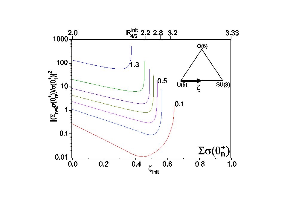
17. E0s, Two nucleon transfer

18. Two Nucleon Transfer Reactions: A New Interpretation for Phase Transitional Regions and Collective Nuclei

19. Empirical survey of (p,t) reaction strengths to 0 + states X O Nearly always: cross sections to excited 0 + states are a small percentage of the ground state cross section. In the spherical – deformed transition region at N = 90, excited state cross sections are comparable to those of the ground state.

20. The “standard interpretation” (since ca. 1960s) of 2-nucleon transfer reactions to excited 0 + states in collective nuclei Most nuclei: Cross sections are small because the collective components add coherently for the ground state but cancel for the orthogonal excited states. (Special (“hot”) single particle orbits can give up to ~20% of the g.s, cross section.) Phase transition region: Spherical and deformed states coexist and mix. Hence a reaction such as (p,t) on a deformed 156 Gd target populates both the “quasi-deformed” ground and “quasi-spherical” excited states of 154 Gd. Well-known signature of phase transitions.

21. Symmetry Triangle of the IBA Sph. Def. Shape/phase trans.

22. The IBA: convenient model that spans the entire triangle of colllective structures The IBA: convenient model that spans the entire triangle of colllective structures  H = ε n d -  Q  Q Parameters: ,  (within Q)  /ε  Sph. DrivingDef. Driving H = c [ ζ ( 1 – ζ ) n d 4N B Q χ ·Q χ - ] Competition: : 0 to infinity  /ε Span triangle with  and  Parameters already known for many nuclei c is an overall scale factor giving the overall energy scale. Normally, it is fit to the first 2 + state.

23. IBA well-suited to this: embodies wide range of collective structures and, being based on s and d bosons, naturally contains an appropriate transfer operator for L=0 -- s-boson Parameters for initial, final nuclei known so calculations are parameter-free Look at Hf isotopes as an example: Exp – all excited state cross sections are small

24. Gd Isotopes: Undergo rapid shape transition at N=90. Excited state cross sections are comparable to g.s.

25. Sph. Def. Shape/phase trans. line ~ 10 5 calculations Big Small So, the model works well and can be used to look at predictions for 2-nucleon transfer strengths Expect: Let’s see what we get !

26. Huh !!???

28. Nuclear Model Codes at Yale Computer name: Titan Connecting to SSH: Quick connect Host name: titan.physics.yale.edu User name: phy664 Port Number 22 Password: nuclear_codes cd phintm pico filename.in (ctrl x, yes, return) runphintm filename (w/o extension) pico filename.out (ctrl x, return)

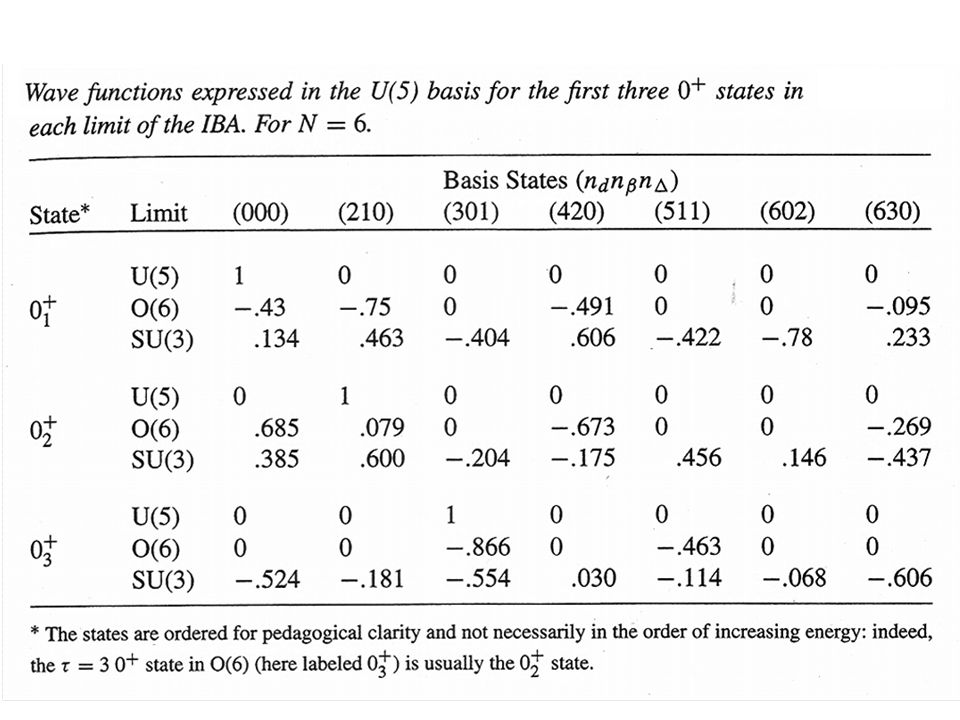
29. The following slides show the IBA input files and partial output files for U(5), SU(3) and O(6)

31. Input $diag eps = 0.20, kappa = 0.00, chi =-0.00, nphmax = 6, iai = 0, iam = 6, neig = 3, mult=.t.,ell=0.0,pair=0.0,oct=0.0,ippm=1,print=.t. $ $em E2SD=1.0, E2DD=-0.00 $ SLCT 2 2+ 0+ 2 99999 Output --------------------------- L P = 0+ Basis vectors |NR> = |ND,NB,NC,LD,NF,L P> --------------------------- | 1> = | 0, 0, 0, 0, 0, 0+> | 2> = | 2, 1, 0, 0, 0, 0+> | 3> = | 3, 0, 1, 0, 0, 0+> | 4> = | 4, 2, 0, 0, 0, 0+> | 5> = | 5, 1, 1, 0, 0, 0+> | 6> = | 6, 0, 2, 0, 0, 0+> | 7> = | 6, 3, 0, 0, 0, 0+> Energies 0.0000 0.4000 0.6000 0.8000 1.0000 1.2000 1.2000 Eigenvectors 1: 1.000 0.000 0.000 2: 0.000 1.000 0.000 3: 0.000 0.000 1.000 4: 0.000 0.000 0.000 5: 0.000 0.000 0.000 6: 0.000 0.000 0.000 7: 0.000 0.000 0.000 --------------------------- L P = 1+ No states --------------------------- L P = 2+ Energies 0.2000 0.4000 0.6000 0.8000 0.8000 1.0000 1.0000 1.2000 1.2000 --------------------------- L P = 3+ Energies 0.6000 1.0000 1.2000 --------------------------- L P = 4+ Energies 0.4000 0.6000 0.8000 0.8000 1.0000 1.0000 1.2000 1.2000 1.2000 --------------------------- L P = 5+ Energies 0.8000 1.0000 1.2000 --------------------------- L P = 6+ Energies 0.6000 0.8000 1.0000 1.0000 1.2000 1.2000 1.2000 -------------------------- Transitions: 2+ -> 0+ (BE2) 2+,1 -> 0+,1: 6.00000 2+,1 -> 0+,2: 2.00000 2+,1 -> 0+,3: 0.00000 2+,2 -> 0+,1: 0.00000 2+,2 -> 0+,2: 0.00000 2+,2 -> 0+,3: 2.40000 2+,3 -> 0+,1: 0.00000 2+,3 -> 0+,2: 5.60000 2+,3 -> 0+,3: 0.00000 and 0+ -> 2+ (BE2) 0+,1 -> 2+,1: 30.00000 0+,2 -> 2+,1: 10.00000 0+,3 -> 2+,1: 0.00000 0+,1 -> 2+,2: 0.00000 0+,2 -> 2+,2: 0.00000 0+,3 -> 2+,2: 12.00000 0+,1 -> 2+,3: 0.00000 0+,2 -> 2+,3: 28.00000 0+,3 -> 2+,3: 0.00000 Transitions: 4+ -> 2+ (BE2) 4+,1 -> 2+,1: 10.00000 4+,1 -> 2+,2: 0.00000 4+,1 -> 2+,3: 2.28571 4+,2 -> 2+,1: 0.00000 4+,2 -> 2+,2: 6.28571 4+,2 -> 2+,3: 0.00000 4+,3 -> 2+,1: 0.00000 4+,3 -> 2+,2: 0.00000 4+,3 -> 2+,3: 3.85714 U(5) Basis Energies Pert. Wave Fcts. U(5) in U(5) basis

32. ******************** Input file contents ******************** $diag eps = 0.00, kappa = 0.02, chi =-1.3229, nphmax = 6, iai = 0, iam = 6, neig = 5, mult=.t.,ell=0.0,pair=0.0,oct=0.0,ippm=1,print=.t. $ $em E2SD=1.0, E2DD=-2.598 $ 99999 ************************************************************* --------------------------- L P = 0+ Basis vectors |NR> = |ND,NB,NC,LD,NF,L P> --------------------------- | 1> = | 0, 0, 0, 0, 0, 0+> | 2> = | 2, 1, 0, 0, 0, 0+> | 3> = | 3, 0, 1, 0, 0, 0+> | 4> = | 4, 2, 0, 0, 0, 0+> | 5> = | 5, 1, 1, 0, 0, 0+> | 6> = | 6, 0, 2, 0, 0, 0+> | 7> = | 6, 3, 0, 0, 0, 0+> Energies 0.0000 0.6600 1.0800 1.2600 1.2600 1.5600 1.8000 Eigenvectors 1: 0.134 0.385 -0.524 -0.235 0.398 2: 0.463 0.600 -0.181 0.041 -0.069 3: -0.404 -0.204 -0.554 -0.557 -0.308 4: 0.606 -0.175 0.030 -0.375 -0.616 5: -0.422 0.456 -0.114 0.255 -0.432 6: -0.078 0.146 -0.068 0.245 -0.415 7: 0.233 -0.437 -0.606 0.606 0.057 --------------------------- L P = 1+ No states --------------------------- L P = 2+ Energies 0.0450 0.7050 0.7050 1.1250 1.1250 1.3050 1.3050 1.6050 --------------------------- L P = 3+ Energies 0.7500 1.1700 1.6500 --------------------------- L P = 4+ Energies 0.1500 0.8100 0.8100 1.2300 1.2300 1.2300 1.4100 1.4100 --------------------------- L P = 5+ Energies 0.8850 1.3050 1.3050 --------------------------- L P = 6+ Energies 0.3150 0.9750 0.9750 1.3950 1.3950 1.5750 1.5750 --------------------------- Binding energy = -1.2000, eps-eff = -0.1550 SU(3) SU(3) wave fcts. in U(5) basis