Download presentation
Presentation is loading. Please wait.

2
Presented by: Erik Cox, Shannon Hintzman, Mike Miller, Jacquie Otto, Adam Serdar, Lacie Zimmerman

3
What’s to come… -Brief history and background of quantum mechanics and quantum computation -Linear Algebra required to understand quantum mechanics -Dirac Bra-ket Notation -Modeling quantum mechanics and applying it to quantum computation

4
History of Quantum Mechanics Sufficiently describes everyday things and events. Breaks down for very small sizes (quantum mechanics) and very high speeds (theory of relativity). Classical (Newtonian) Physics
 and very high speeds (theory of relativity). Classical (Newtonian) Physics.")
5
Why do we need Quantum Mechanics? In short, quantum mechanics describes behaviors that classical (Newtonian) physics cannot. Some behaviors include: - The wave-particle duality of light and matter - Discreteness of energy - Quantum tunneling - The Heisenberg uncertainty principle - Spin of a particle
 physics cannot. Some behaviors include: - The wave-particle duality of light and matter - Discreteness of energy - Quantum tunneling - The Heisenberg uncertainty principle - Spin of a particle.")
6
Spin of a Particle - Discovered in 1922 by Otto Stern and Walther Gerlach - Experiment indicated that atomic particles possess intrinsic angular momentum, called spin, that can only have certain discrete values.

7
The Quantum Computer Idea developed by Richard Feynman in 1982. Concept: Create a computer that uses the effects of quantum mechanics to its advantage.

8
Classical Computer Information Quantum Computer Information vs. - Bit, exists in two states, 0 or 1 - Qubit, exists in two states, 0 or 1, and superposition of both

9
Why are quantum computers important? Recently, Peter Shor developed an algorithm to factor large numbers on a quantum computer. Since factoring is key to current encryption, quantum computers would be able to quickly break current cryptography techniques.

10
In the beginning, there was Linear Algebra… - Complex inner product spaces - Linear Operators - Unitary Operators - Projections - Tensor Products

11
Complex inner product spaces An inner product space is a complex vector space, together with a map f : V x V → F where F is the ground field C. We write instead of f(x, y) and require that the following axioms be satisfied:
 and require that the following axioms be satisfied:.")
12
and iff denotes complex conjugate (Positive Definiteness) (Conjugate Bilinearity) (Conjugate Symmetry)
 (Conjugate Bilinearity) (Conjugate Symmetry)")
13
Complex Conjugate: where Example of Complex Inner Product Space: Let

14
Linear Operators Example: (Additivity) (Homogeneity) Let and be vector spaces over, then is a linear operator if. The following properties exist:

15
Unitary Operators t denotes adjoint Properties: Norm Preserving… Inner Product Preserving…

16
Adjoints Matrix Representation

17
Suppose Definition of Adjoint: (Inner Product Preserving) (Norm Preserving)
 (Norm Preserving)")
18
In quantum mechanics we use orthogonal projections. Definition: Let V be an inner product space over F. Let M be a subspace of V. Given an element then the orthogonal projection of y onto M is the vector which satisfies where v is orthogonal to every element.

19
A projection operator P on V satisfies We say P is the projection onto its range, i.e., onto the subspace

20
In quantum mechanics tensor products are used with : Vectors Vector Spaces Operators N-Fold tensor products.

21
If and, there is a natural mapping defined by We use notation w v to symbolize T(w, v) and call w v the tensor product of w and v.
 and call w v the tensor product of w and v.")
22
W V means the vector space consisting of all finite formal sums: where and

23
If A, B are operators on W and V we define A B on W V by

24
4 Properties of Tensor Products 1.a(w v) = (aw) v = w (av) for all a in C; 2.(x + y) v = x v + y v; 3.w (x + y) = w x + w y; 4. w x | y z = w | y x | v . Note: | is the notation used for inner products in quantum mechanics.

25
Property #1: a(w v) = (aw) v = w (av) for all a in C Example in :
 = (aw) v = w (av) for all a in C Example in :")
26
Example in :

28
Property #2: (x + y) v = x v + y v Example in :
 v = x v + y v Example in :")
30
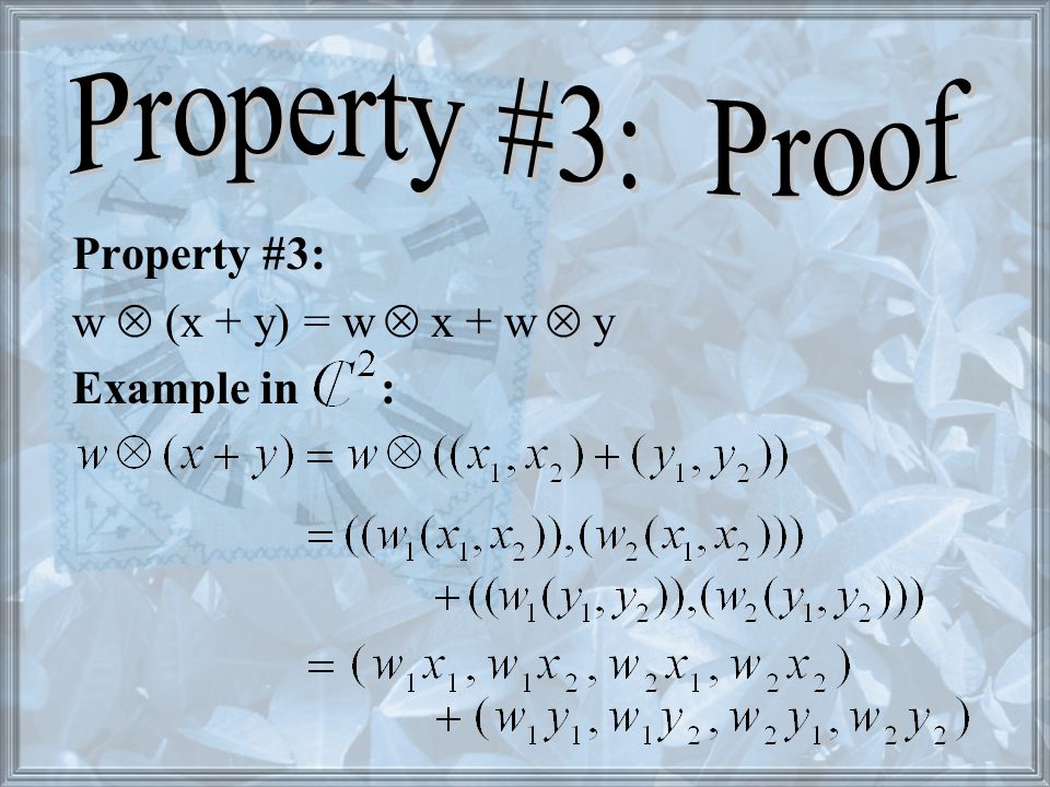
Property #3: w (x + y) = w x + w y Example in :
 = w x + w y Example in :")
32
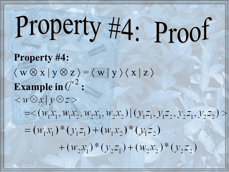
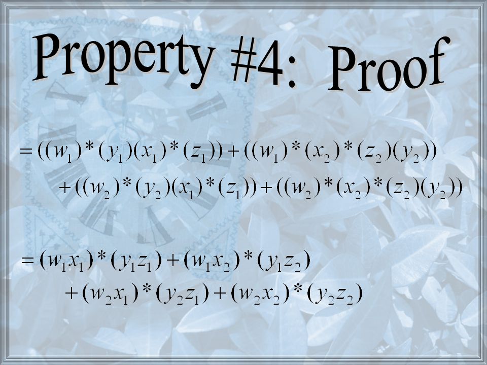
Property #4: w x | y z = w | y x | z Example in :

35
Dirac Bra-Ket Notation Notation Inner Products Outer Products Completeness Equation Outer Product Representation of Operators

36
Bra-Ket Notation Involves Bra t Ket |n> Vector X n can be represented two ways is the complex conjugate of m

37
Inner Products An Inner Product is a Bra multiplied by a Ket can be simplified to = =

38
Outer Products An Outer Product is a Ket multiplied by a Bra |y><x| == By Definition

39
Completeness Equation So Effectively Let |i>, i = 1, 2,..., n, be a basis for V and v is a vector in V is used to create a identity operator represented by vector products.

40
Proof for the Completeness Equation Using Linear Algebra, the basis of a vectors space can be represented series of vectors with a one in each successive position and zeros in every other (aka {1, 0, 0,... }, {0, 1, 0,...}, {0, 0, 1,...},...) So |i><i| will create a matrix with a one in each successive position along the diagonal. etc.
 So |i><i| will create a matrix with a one in each successive position along the diagonal. etc..")
41
Completeness Cont. Thus = +++... = = I

42
One application of the Dirac notation is to represent Operators in terms of inner and outer products. and

43
If A is an operator, we can represent A by applying the completeness equation twice this gives the following equation: This shows that any operator has an outer product representation and that the entries of the associated matrix for the basis |i are:

44
Projections Projection is a type of operator Application of inner and outer products

45
Linear Algebra View We can represent graphically: Using the rule of dot products we know Given that we can say

46
Linear Algebra View (Cont.) Using these facts we can solve for and Again using the rule of dot products We get
 Using these facts we can solve for and Again using the rule of dot products We get")
47
Linear Algebra View (Cont.) So Plugging this back into the original equation Gives us:
 So Plugging this back into the original equation Gives us:")
48
Linear Algebra View (Cont.) If is a unit vector
 If is a unit vector")
49
Projections in Quantum Mechanics Given that and This graph is a representation of Given and

50
Projections in QM (cont.) being the full basis of We can regard the full basis of as being On Basis For some
 being the full basis of We can regard the full basis of as being On Basis For some")
51
Projections in QM (cont.) Taking the inner products gives Therefore and more generally So
 Taking the inner products gives Therefore and more generally So")
52
Projections in QM (cont.) Now set So
 Now set So")
53
Computational Basis Basis for

54
Computational Basis (cont.) A basis for will have basis vectors: Called a computational basis Notation:
 A basis for will have basis vectors: Called a computational basis Notation:")
55
Quantum States Thinking in terms of directions model quantum states by directions in a vector space

57
Associated with an isolated quantum system is an inner product space called the “state space” of the system. The system at any given time is described by a “state”, which is a unit vector in V.

58
Simplest state space - or Qubit If and form a basis for, then an arbitrary qubit state has the form, where a and b in have. Qubit state differs from a bit because “superpositions” of an arbitrary qubit state are possible.

59
The evolution of an isolated quantum system is described by a unitary operator on its state space. The state is related to the state by a unitary operator i.e.,.

60
Quantum measurements are described by a finite set, {P m }, of projections acting on the state space of the system being measured.

61
If the state of the system is immediately before the measurement, then the probability that the result m occurs is given by.

62
If the result m occurs, then the state of the system immediately after the measurement is

63
The state space of a composite quantum system is the tensor product of the state of its components. If the systems numbered 1 through n are prepared in states, i = 1,…, n, then the joint state of the composite total system is.

64
Product vs. Entangled States Product State – a state in V n is called a product state if it has the form: Entangled State – if is a linear combination of that can’t be written as a product state

65
Example of an Entangled State The 2-qubit in the state Suppose: |00 + |11 = |a |b for some |a and |b . Taking inner products with |00 , |11 , and |01 and applying the state space property of tensor products (states | i , i=1, …, n, then the joint state of the composite total system is | 1 · · · | n ) gives 0|a 0|b = 1, 1|a 1|b = 1, and 0|a 1|b = 0, respectively. Since neither 0|a nor 1|b is 0, this gives a contradiction
 gives 0|a 0|b = 1, 1|a 1|b = 1, and 0|a 1|b = 0, respectively. Since neither 0|a nor 1|b is 0, this gives a contradiction.")
66
Tying it all Together With an example of a 2-qubit

67
Example of a 2-qubit A qubit is a 2-dimensional quantum system (say a photon) and a 2-qubit is a composite of two qubits 2-qubits “live” in the vector space
 and a 2-qubit is a composite of two qubits 2-qubits live in the vector space")
68
Suppose that is an example of a 2 component system with being a linear combination of basic qubits with amplitude being the coefficients: In which

69
Measuring the 1 st qubit When we measure the first qubit in the composite system, the measuring apparatus interacts with the 1 st qubit and leaves the 2 nd qubit undisturbed (postulate 4), similarly when we measure the 2 nd qubit the measuring device leaves the 1 st qubit undisturbed Thus, we apply the measurement,in which
, similarly when we measure the 2 nd qubit the measuring device leaves the 1 st qubit undisturbed Thus, we apply the measurement,in which")
70
Leading to the probabilities and post measurement states… Using postulate 3 the probability that 0 occurs is given by If the result 0 occurs, then the state of the system immediately after the measurement is given by

71
Similarly we obtain the result 1 on the 1 st qubit with probability… Resulting in the post-measurement state…

72
In the same way for the second qubit…

73
Consider the entangled 2-qubit

74
We consider with amplitudes

75
After applying Quantum Measurement Techniques the post measurement states are (A Perfectly Correlated Measurement) The probabilities for each state for each qubit are all 1/2
 The probabilities for each state for each qubit are all 1/2")
76
Conclusion Brief History of Quantum Mechanics Tools Of Linear Algebra –Complex Inner Product Spaces –Linear and Unitary Operators –Projections –Tensor Products

77
Conclusion Cont. Dirac Bra-Ket Notation –Inner and Outer Products –Completeness Equation –Outer Product Representations –Projections –Computational Bases

78
Conclusion Cont. (again) Mathematical Model of Quantum Mech. –Quantum States –Postulates of Quantum Mechanics –Product vs. Entangled States

79
Where do we go from here? Quantum Circuits Superdense Coding and Teleportation

80
Bibliography http://en.wikipedia.org/wiki/Inner_product_space http://vergil.chemistry.gatech.edu/notes/quantrev/node14.html http://en2.wikipedia.org/wiki/Linear_operator http://vergil.chemistry.gatech.edu/notes/quantrev/node17.html http://www.doc.ic.ad.uk/~nd/surprise_97/journal/vol4/spb3/ http://www-theory.chem.washington.edu/~trstedl/quantum/quantum.html Gudder, S. (2003-March). Quantum Computation. American Mathmatical Monthly. 110, no. 3,181-188. Special Thanks to: Dr. Steve Deckelman Dr. Alan Scott
. Quantum Computation. American Mathmatical Monthly. 110, no. 3, Special Thanks to: Dr. Steve Deckelman Dr. Alan Scott.")
Similar presentations


![Xkcd Xkcd.com. Section 3 Recap ► Angular momentum commutators: [J x, J y ] = iħJ z etc ► Total ang. Mom. Operator: J 2 = J x 2 + J y 2 +J z 2 ► Ladder.](/8/2429168/big_thumb.jpg "Xkcd Xkcd.com. Section 3 Recap ► Angular momentum commutators: [J x, J y ] = iħJ z etc ► Total ang. Mom. Operator: J 2 = J x 2 + J y 2 +J z 2 ► Ladder.>")


 are.>")