Download presentation
Presentation is loading. Please wait.

1
Quantum One: Lecture 9

3
Graham Schmidt Orthogonalization

4
In the last lecture, we extended out definitions of spanning sets, linearly independent sets, and basis sets to allow an application of these concepts to continuously indexed sets of vectors. We then introduced the idea of an inner product, which extends to complex vectors spaces the familiar dot product encountered in real vector spaces. This allowed us to define the norm or length of a vector, to define unit vectors, and to introduce a limited notion of direction through the concept of orthogonality. These notions of length, and orthogonality, allowed us to define orthonormal sets of vectors, with either discrete or continuous indices, and to end up with the idea of an orthonormal basis, i.e., an orthonormal set of vectors that span the space.

5
In this lecture we begin by showing that it is always possible to construct an orthonormal basis set from any set of basis vectors of finite length. The explicit algorithm for doing so, referred to as the Gram-Schmidt orthogonalization procedure, is presented below.

6
Let be a set of linearly independent vectors of finite length. 1. Set This produces a unit vector |φ₁ 〉 pointing along the same direction as |χ₁ 〉. Now construct a second vector orthogonal to the first, by subtracting off that part of it which lies along the direction of the first vector: 2. Set Note, that by construction so |ψ₂ 〉 and thus |φ₂ 〉 are orthogonal to |φ₁ 〉.

7
Let be a set of linearly independent vectors of finite length. 1. Set This produces a unit vector |φ₁ 〉 pointing along the same direction as |χ₁ 〉. Now construct a second vector orthogonal to the first, by subtracting off that part of it which lies along the direction of the first vector: 2. Set Note, that by construction so |ψ₂ 〉 and thus |φ₂ 〉 are orthogonal to |φ₁ 〉.

8
Let be a set of linearly independent vectors of finite length. 1. Set This produces a unit vector |φ₁ 〉 pointing along the same direction as |χ₁ 〉. Now construct a second vector orthogonal to the first, by subtracting off that part of it which lies along the direction of the first vector: 2. Set Note, that by construction so |ψ₂ 〉 and thus |φ₂ 〉 are orthogonal to |φ₁ 〉.

9
Let be a set of linearly independent vectors of finite length. 1. Set This produces a unit vector |φ₁ 〉 pointing along the same direction as |χ₁ 〉. Now construct a second vector orthogonal to the first, by subtracting off that part of it which lies along the direction of the first vector: 2. Set Note, that by construction so |ψ₂ 〉 and thus |φ₂ 〉 are orthogonal to |φ₁ 〉.

10
Let be a set of linearly independent vectors of finite length. 1. Set This produces a unit vector |φ₁ 〉 pointing along the same direction as |χ₁ 〉. Now construct a second vector orthogonal to the first, by subtracting off that part of it which lies along the direction of the first vector: 2. Set Note, that by construction so |ψ₂ 〉 and thus |φ₂ 〉 are orthogonal to |φ₁ 〉.

11
Let be a set of linearly independent vectors of finite length. 1. Set This produces a unit vector |φ₁ 〉 pointing along the same direction as |χ₁ 〉. Now construct a second vector orthogonal to the first, by subtracting off that part of it which lies along the direction of the first vector: 2. Set Note, that by construction so |ψ₂ 〉 and thus |φ₂ 〉 are orthogonal to |φ₁ 〉.

12
Let be a set of linearly independent vectors of finite length. 1. Set This produces a unit vector |φ₁ 〉 pointing along the same direction as |χ₁ 〉. Now construct a second vector orthogonal to the first, by subtracting off that part of it which lies along the direction of the first vector: 2. Set Note, that by construction so |ψ₂ 〉 and thus |φ₂ 〉 are orthogonal to |φ₁ 〉.

13
We now proceed in this fashion, constructing each new vector orthogonal to each of those previously constructed. Thus, 3. Set and, at the nth step Set so that

14
We now proceed in this fashion, constructing each new vector orthogonal to each of those previously constructed. That is we 3. Set and, at the nth step Set so that

15
We now proceed in this fashion, constructing each new vector orthogonal to each of those previously constructed. Thus, 3. Set and, at the nth step Set so that

16
We now proceed in this fashion, constructing each new vector orthogonal to each of those previously constructed. Thus, 3. Set and, at the nth step Set so that

17
We now proceed in this fashion, constructing each new vector orthogonal to each of those previously constructed. Thus, 3. Set and, at the nth step Set so that

18
We now proceed in this fashion, constructing each new vector orthogonal to each of those previously constructed. Thus, 3. Set and, at the nth step Set so that

19
The only way this process could stop is if one of the resulting vectors turned out to be the null vector. A close inspection of the process reveals that this can't happen if the original set is linearly independent, as we have assumed. Thus, in this way we can construct an orthonormal set of vectors equal in number to those of the original set. It follows, that given any basis for the space we can construct an orthonormal basis with an equal number of vectors. In the next lecture, we figure out why that’s a very good thing.

20
The only way this process could stop is if one of the resulting vectors turned out to be the null vector. A close inspection of the process reveals that this can't happen if the original set is linearly independent, as we have assumed. Thus, in this way we can construct an orthonormal set of vectors equal in number to those of the original set. It follows, that given any basis for the space we can construct an orthonormal basis with an equal number of vectors. In the next lecture, we figure out why that’s a very good thing.

21
The only way this process could stop is if one of the resulting vectors turned out to be the null vector. A close inspection of the process reveals that this can't happen if the original set is linearly independent, as we have assumed. Thus, in this way we can construct an orthonormal set of vectors equal in number to those of the original set. It follows, that given any basis for the space we can construct an orthonormal basis with an equal number of vectors. In the next lecture, we figure out why that’s a very good thing.

22
The only way this process could stop is if one of the resulting vectors turned out to be the null vector. A close inspection of the process reveals that this can't happen if the original set is linearly independent, as we have assumed. Thus, in this way we can construct an orthonormal set of vectors equal in number to those of the original set. It follows, that given any basis for the space we can construct an orthonormal basis with an equal number of vectors. We now explore how orthonormal bases make our lives easier.

24
Expansion of a Vector on an Orthonormal Basis

25
Discrete Bases - Let the set form an orthonormal basis (or ONB) for the space S, so that and let |χ 〉 be an arbitrary element of the space. By assumption there exists an expansion of the form for a unique set of expansion coefficients. Q: How do we determine what these expansion coefficients are?

26
Discrete Bases - Let the set form an orthonormal basis (or ONB) for the space S, so that and let |χ 〉 be an arbitrary element of the space. By assumption there exists an expansion of the form for a unique set of expansion coefficients. Q: How do we determine what these expansion coefficients are?

27
Discrete Bases - Let the set form an orthonormal basis (or ONB) for the space S, so that and let |χ 〉 be an arbitrary element of the space. By assumption there exists an expansion of the form for a unique set of expansion coefficients. Q: How do we determine what these expansion coefficients are?

28
Discrete Bases - Let the set form an orthonormal basis (or ONB) for the space S, so that and let |χ 〉 be an arbitrary element of the space. By assumption there exists an expansion of the form for a unique set of expansion coefficients. Question: How do we determine what these expansion coefficients are?

29
Consider the inner product of the vector |χ 〉 with an arbitrary element of this basis: This shows that the expansion coefficient is just the inner product of the vector we are expanding with the unit vector along that direction in Hilbert space. Thus, expansion coefficient = inner product with basis vector

30
Consider the inner product of the vector |χ 〉 with an arbitrary element of this basis: This shows that the expansion coefficient is just the inner product of the vector we are expanding with the unit vector along that direction in Hilbert space. Thus, expansion coefficient = inner product with basis vector

31
Consider the inner product of the vector |χ 〉 with an arbitrary element of this basis: This shows that the expansion coefficient is just the inner product of the vector we are expanding with the unit vector along that direction in Hilbert space. Thus, expansion coefficient = inner product with basis vector

32
Consider the inner product of the vector |χ 〉 with an arbitrary element of this basis: This shows that the expansion coefficient is just the inner product of the vector we are expanding with the unit vector along that direction in Hilbert space. Thus, expansion coefficient = inner product with basis vector

33
Consider the inner product of the vector |χ 〉 with an arbitrary element of this basis: This shows that the expansion coefficient is just the inner product of the vector we are expanding with the unit vector along that direction in Hilbert space. Thus, expansion coefficient = inner product with basis vector

34
Consider the inner product of the vector |χ 〉 with an arbitrary element of this basis: This shows that the expansion coefficient is just the inner product of the vector we are expanding with the unit vector along that direction in Hilbert space. Thus, We can then write the expansion as

35
Consider the inner product of the vector |χ 〉 with an arbitrary element of this basis: This shows that the expansion coefficient is just the inner product of the vector we are expanding with the unit vector along that direction in Hilbert space. Thus, We can then write the expansion as

36
Extension to Continuous Bases - Let the set form an orthonormal basis (or ONB) for the space S, so that and let |χ 〉 be an arbitrary element of the space. By assumption there exists an expansion of the form for some unique expansion function. Q: How do we determine what this expansion function is?

37
Extension to Continuous Bases - Let the set form an orthonormal basis (or ONB) for the space S, so that and let |χ 〉 be an arbitrary element of the space. By assumption there exists an expansion of the form for some unique expansion function. Q: How do we determine what this expansion function is?

38
Extension to Continuous Bases - Let the set form an orthonormal basis (or ONB) for the space S, so that and let |χ 〉 be an arbitrary element of the space. By assumption there exists an expansion of the form for some unique expansion function. Q: How do we determine what this expansion function is?

39
Extension to Continuous Bases - Let the set form an orthonormal basis (or ONB) for the space S, so that and let |χ 〉 be an arbitrary element of the space. By assumption there exists an expansion of the form for some unique expansion function. Q: How do we determine what this expansion function is?

40
Extension to Continuous Bases - Let the set form an orthonormal basis (or ONB) for the space S, so that and let |χ 〉 be an arbitrary element of the space. By assumption there exists an expansion of the form for some unique expansion function. Question: How do we determine what this expansion function is?

41
Consider the inner product of the vector |χ 〉 with an arbitrary element of this basis: This shows that the expansion coefficient is just the inner product of the vector we are expanding with the unit vector along that direction in Hilbert space. Thus, expansion coefficient = inner product with basis vector

42
Consider the inner product of the vector |χ 〉 with an arbitrary element of this basis: This shows that the expansion coefficient is just the inner product of the vector we are expanding with the unit vector along that direction in Hilbert space. Thus, expansion coefficient = inner product with basis vector

43
Consider the inner product of the vector |χ 〉 with an arbitrary element of this basis: This shows that the expansion coefficient is just the inner product of the vector we are expanding with the unit vector along that direction in Hilbert space. Thus, expansion coefficient = inner product with basis vector

44
Consider the inner product of the vector |χ 〉 with an arbitrary element of this basis: This shows that the expansion coefficient is just the inner product of the vector we are expanding with the unit vector along that direction in Hilbert space. Thus, expansion coefficient = inner product with basis vector

45
Consider the inner product of the vector |χ 〉 with an arbitrary element of this basis: This shows that the expansion coefficient is just the inner product of the vector we are expanding with the unit vector along that direction in Hilbert space. Thus, expansion coefficient = inner product with basis vector

46
Consider the inner product of the vector |χ 〉 with an arbitrary element of this basis: This shows that the expansion coefficient is just the inner product of the vector we are expanding with the unit vector along that direction in Hilbert space. Thus, expansion coefficient = inner product with basis vector

47
Consider the inner product of the vector |χ 〉 with an arbitrary element of this basis: This shows that the expansion coefficient is just the inner product of the vector we are expanding with the unit vector along that direction in Hilbert space. Thus,

48
So: where We will refer to the function χ(α) as the "wave function" representing |χ 〉 in the α representation. Note: This expansion can also be written in the suggestive the form

49
So: where We will refer to the function χ(α) as the "wave function" representing |χ 〉 in the α representation. Note: This expansion can also be written in the suggestive the form

50
So: where We will refer to the function χ(α) as the "wave function" representing |χ 〉 in the α representation. Note: This expansion can also be written in the suggestive form

51
So: where We will refer to the function χ(α) as the "wave function" representing |χ 〉 in the α representation. Note: This expansion can also be written in the suggestive form

52
A Notational Simplification: It is clear that when we talk about ONB's, such as 〉 } or, the important information which distinguishes the different basis vectors from one another is the label or index: i or j in the discrete case, α or α′ in the continuous case. The symbols φ just sort of come along for the ride, a historical vestige of when we were expanded in sets of functions. From this point on we will acknowledge this by using an abbreviated notation: and In this way the expansions of an arbitrary ket can be written and

53
A Notational Simplification: It is clear that when we talk about ONB's, such as 〉 } or, the important information which distinguishes the different basis vectors from one another is the label or index: i or j in the discrete case, α or α′ in the continuous case. The symbols φ just sort of come along for the ride, a historical vestige of when we were expanded in sets of functions. From this point on we will acknowledge this by using an abbreviated notation: and In this way the expansions of an arbitrary ket can be written and

54
A Notational Simplification: It is clear that when we talk about ONB's, such as 〉 } or, the important information which distinguishes the different basis vectors from one another is the label or index: i or j in the discrete case, α or α′ in the continuous case. The symbols φ just sort of come along for the ride, a historical vestige of when we were expanding in sets of functions. From this point on we will acknowledge this by using an abbreviated notation: and In this way the expansions of an arbitrary ket can be written and

55
A Notational Simplification: It is clear that when we talk about ONB's, such as 〉 } or, the important information which distinguishes the different basis vectors from one another is the label or index: i or j in the discrete case, α or α′ in the continuous case. The symbols φ just sort of come along for the ride, a historical vestige of when we were expanding in sets of functions. From this point on we will acknowledge this by using an abbreviated notation: and In this way the expansions of an arbitrary ket can be written and

56
A Notational Simplification: It is clear that when we talk about ONB's, such as 〉 } or, the important information which distinguishes the different basis vectors from one another is the label or index: i or j in the discrete case, α or α′ in the continuous case. The symbols φ just sort of come along for the ride, a historical vestige of when we were expanding in sets of functions. From this point on we will acknowledge this by using an abbreviated notation: and In this way the expansions of an arbitrary ket can be written and

57
A Notational Simplification: It is clear that when we talk about ONB's, such as 〉 } or, the important information which distinguishes the different basis vectors from one another is the label or index: i or j in the discrete case, α or α′ in the continuous case. The symbols φ just sort of come along for the ride, a historical vestige of when we were expanded in sets of functions. From this point on we will acknowledge this by using an abbreviated notation: and In this way the expansions of an arbitrary ket can be written and

58
A Notational Simplification: It is clear that when we talk about ONB's, such as 〉 } or, the important information which distinguishes the different basis vectors from one another is the label or index: i or j in the discrete case, α or α′ in the continuous case. The symbols φ just sort of come along for the ride, a historical vestige of when we were expanding in sets of functions. From this point on we will acknowledge this by using an abbreviated notation: and In this way the expansions of an arbitrary ket can be written and

60
Calculation of Inner Products Using an Orthonormal Basis

62
The Emergence of Numerical Representations

63
Discrete Bases - Let the set form an orthonormal basis for S, so that and let |χ 〉 and |ψ 〉 be arbitrary states of S. These states can be expanded in this basis set Suppose we know these expansion coefficients, and we want to know the inner product of these two vectors.

64
Discrete Bases - Let the set form an orthonormal basis for S, so that and let |χ 〉 and |ψ 〉 be arbitrary states of S. These states can be expanded in this basis set Suppose we know these expansion coefficients, and we want to know the inner product of these two vectors.

65
Discrete Bases - Let the set form an orthonormal basis for S, so that and let |χ 〉 and |ψ 〉 be arbitrary states of S. These states can be expanded in this basis set Suppose we know these expansion coefficients, and we want to know the inner product of these two vectors.

66
Discrete Bases - Let the set form an orthonormal basis for S, so that and let |χ 〉 and |ψ 〉 be arbitrary states of S. These states can be expanded in this basis set Suppose we know these expansion coefficients, and we want to know the inner product of these two vectors.

67
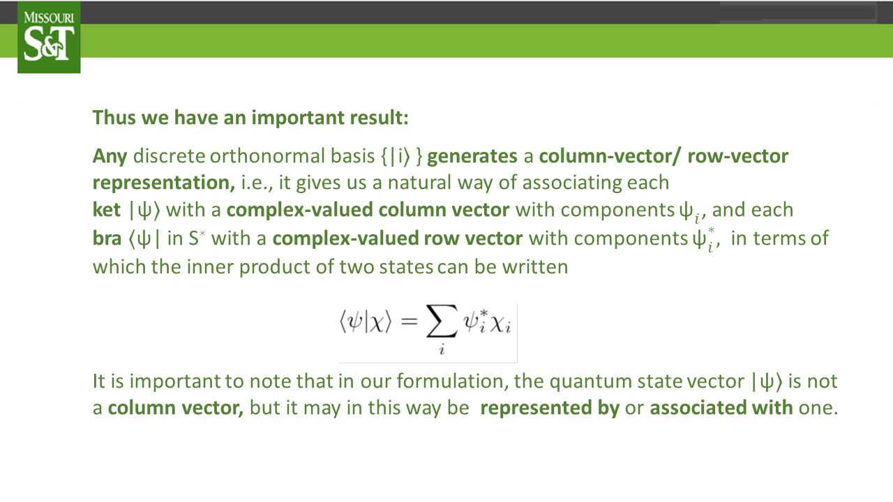
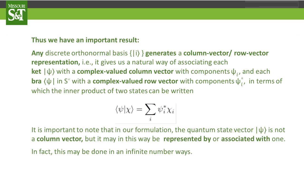
Well, we can express the desired inner product in the form But So we can write this inner product in the form But this is exactly of the form of the inner product in in C N

68
Well, we can express the desired inner product in the form But So we can write this inner product in the form But this is exactly of the form of the inner product in in C N

69
Well, we can express the desired inner product in the form But So we can write this inner product in the form But this is exactly of the form of the inner product in in C N

70
Well, we can express the desired inner product in the form But So we can write this inner product in the form But this is exactly of the form of the inner product in in C N

71
Well, we can express the desired inner product in the form But So we can write this inner product in the form But this is exactly of the form of the inner product in in C N

72
Well, we can express the desired inner product in the form But So we can write this inner product in the form But this is exactly of the form of the inner product in C N

76
Continuous Bases - Let the set form a continuous orthonormal basis for S, so that and let |χ 〉 and |ψ 〉 be arbitrary states of S. These states can be expanded in this basis Suppose we know these expansion functions, and we want to know the inner product of these two vectors.

77
Continuous Bases - Let the set form a continuous orthonormal basis for S, so that and let |χ 〉 and |ψ 〉 be arbitrary states of S. These states can be expanded in this basis Suppose we know these expansion functions, and we want to know the inner product of these two vectors.

78
Continuous Bases - Let the set form a continuous orthonormal basis for S, so that and let |χ 〉 and |ψ 〉 be arbitrary states of S. These states can be expanded in this basis Suppose we know these expansion functions, and we want to know the inner product of these two vectors.

79
Continuous Bases - Let the set form a continuous orthonormal basis for S, so that and let |χ 〉 and |ψ 〉 be arbitrary states of S. These states can be expanded in this basis Suppose we know these expansion functions, and we want to know the inner product of these two vectors.

80
Well, we can express the desired inner product in the form But So we can write this inner product in the form But this is exactly of the form of the inner product in functional linear vector spaces

81
Well, we can express the desired inner product in the form But So we can write this inner product in the form But this is exactly of the form of the inner product in functional linear vector spaces

82
Well, we can express the desired inner product in the form But So we can write this inner product in the form But this is exactly of the form of the inner product in functional linear vector spaces

83
Well, we can express the desired inner product in the form But So we can write this inner product in the form But this is exactly of the form of the inner product in functional linear vector spaces

84
Well, we can express the desired inner product in the form But So we can write this inner product in the form But this is exactly of the form of the inner product in functional linear vector spaces

85
Well, we can express the desired inner product in the form But So we can write this inner product in the form But this is exactly of the form of the inner product in functional linear vector spaces

86
Thus we have an important result: Any continuous orthonormal basis {|α 〉 } induces a wave function representation for the space, i.e., it gives us a natural way of associating each ket |ψ 〉 in S with a complex-valued wave function ψ(α) and each bra 〈 ψ| in S ∗ with a complex-valued wave function ψ ∗ (α). We refer to ψ(α) as the wave function for the state |ψ 〉 in the α-representation. In this representation the inner product of two states can be computed as It is important to note that in our formulation, the quantum state vector |ψ 〉 is not a wave function but it may in this way be represented by or associated with one. In fact, this may be done in an infinite number ways.
 as the wave function for the state |ψ 〉 in the α-representation. In this representation the inner product of two states can be computed as It is important to note that in our formulation, the quantum state vector |ψ 〉 is not a wave function but it may in this way be represented by or associated with one. In fact, this may be done in an infinite number ways..")
87
Thus we have an important result: Any continuous orthonormal basis {|α 〉 } induces a wave function representation for the space, i.e., it gives us a natural way of associating each ket |ψ 〉 in S with a complex-valued wave function ψ(α) and each bra 〈 ψ| in S ∗ with a complex-valued wave function ψ ∗ (α). We refer to ψ(α) as the wave function for the state |ψ 〉 in the α-representation. In this representation the inner product of two states can be computed as It is important to note that in our formulation, the quantum state vector |ψ 〉 is not a wave function but it may in this way be represented by or associated with one. In fact, this may be done in an infinite number ways.
 as the wave function for the state |ψ 〉 in the α-representation. In this representation the inner product of two states can be computed as It is important to note that in our formulation, the quantum state vector |ψ 〉 is not a wave function but it may in this way be represented by or associated with one. In fact, this may be done in an infinite number ways..")
88
Thus we have an important result: Any continuous orthonormal basis {|α 〉 } induces a wave function representation for the space, i.e., it gives us a natural way of associating each ket |ψ 〉 in S with a complex-valued wave function ψ(α) and each bra 〈 ψ| in S ∗ with a complex-valued wave function ψ ∗ (α). We refer to ψ(α) as the wave function for the state |ψ 〉 in the α-representation. In this representation the inner product of two states can be computed as It is important to note that in our formulation, the quantum state vector |ψ 〉 is not a wave function but it may in this way be represented by or associated with one. In fact, this may be done in an infinite number ways.
 as the wave function for the state |ψ 〉 in the α-representation. In this representation the inner product of two states can be computed as It is important to note that in our formulation, the quantum state vector |ψ 〉 is not a wave function but it may in this way be represented by or associated with one. In fact, this may be done in an infinite number ways..")
89
Thus we have an important result: Any continuous orthonormal basis {|α 〉 } induces a wave function representation for the space, i.e., it gives us a natural way of associating each ket |ψ 〉 in S with a complex-valued wave function ψ(α) and each bra 〈 ψ| in S ∗ with a complex-valued wave function ψ ∗ (α). We refer to ψ(α) as the wave function for the state |ψ 〉 in the α-representation. In this representation the inner product of two states can be computed as It is important to note that in our formulation, the quantum state vector |ψ 〉 is not a wave function but it may in this way be represented by or associated with one. In fact, this may be done in an infinite number ways.
 as the wave function for the state |ψ 〉 in the α-representation. In this representation the inner product of two states can be computed as It is important to note that in our formulation, the quantum state vector |ψ 〉 is not a wave function but it may in this way be represented by or associated with one. In fact, this may be done in an infinite number ways..")
90
In the next lecture we attempt to make some of these admittedly abstract ideas more concrete, by applying our general formulation of quantum mechanics to the quantum state space of a single quantum mechanical particle. In so doing, we will see how, in a natural and physically meaningful way the “Schrödinger” representation, which associates the quantum state with a wave function, emerges from the formal mathematical structure developed thus far.

91
In the next lecture we attempt to make some of these admittedly abstract ideas more concrete, by applying our general formulation of quantum mechanics to the quantum state space of a single quantum mechanical particle. In so doing, we will see how, in a natural and physically meaningful way the “Schrödinger” representation, which associates the quantum state with a wave function, emerges from the formal mathematical structure developed thus far.

92
In the next lecture we attempt to make some of these admittedly abstract ideas more concrete, by applying our general formulation of quantum mechanics to the quantum state space of a single quantum mechanical particle. In so doing, we will see how, in a natural and physically meaningful way the “Schrödinger” representation, which associates the quantum state with a wave function, emerges from the formal mathematical structure developed thus far.

93
In the next lecture we attempt to make some of these admittedly abstract ideas more concrete, by applying our general formulation of quantum mechanics to the quantum state space of a single quantum mechanical particle. In so doing, we will see how, in a natural and physically meaningful way the “Schrödinger” representation, which associates the quantum state with a wave function, emerges from the formal mathematical structure developed thus far.

Similar presentations