Download presentation
Presentation is loading. Please wait.

1
Earthquake Location The basic principles Relocation methods
S-P location (manual) location by inversion single station location depth assessment velocity models Relocation methods joint hypocentral location master event location Other related topics Waveform modeling Automated phase picking Topic covered in this session
 location by inversion. single station location. depth assessment. velocity models. Relocation methods. joint hypocentral location. master event location. Other related topics. Waveform modeling. Automated phase picking. Topic covered in this session.")
2
Basic Principles 4 unknowns - origin time, x, y, z
Data from seismograms – phase arrival times There are four unknowns in the problem of earthquake location – the origin time of the earthquake and the three geographical co-ordinates of the focus. The data used to resolve these unknowns are the recorded seismograms. The simplest solution comes from considering the phase arrival times. If we have a good velocity model the difference in time between the S and P arrival can be converted into distance.

3
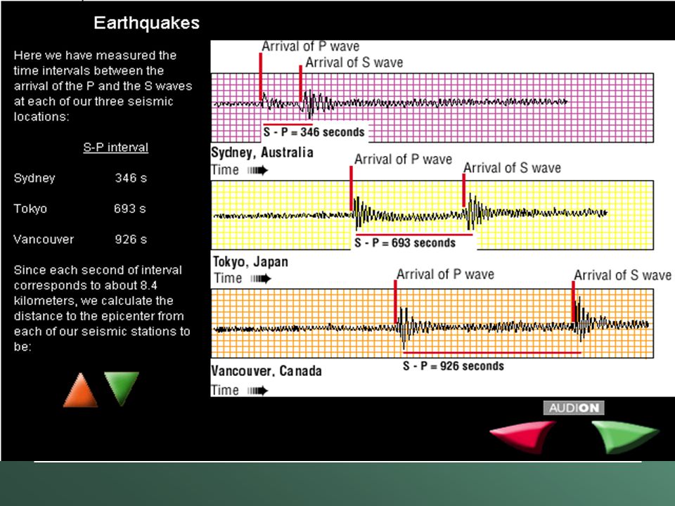
S-P time Time between P and S arrivals increases with distance from the focus. A single trace can therefore give the origin time and distance (but not azimuth) Because P wave velocities are greater than S wave velocities, the separation between the phases increases with distance from the focus. Using this approach each station can be used to estimate the distance from the station to the focus. A rough approximation of the relationship between S-P time and distance is D [in degrees]=8*(S-P) [in minutes] approximates to
 Because P wave velocities are greater than S wave velocities, the separation between the phases increases with distance from the focus. Using this approach each station can be used to estimate the distance from the station to the focus. A rough approximation of the relationship between S-P time and distance is D [in degrees]=8*(S-P) [in minutes] approximates to.")
4
Manual Method

5
Seismogram

12
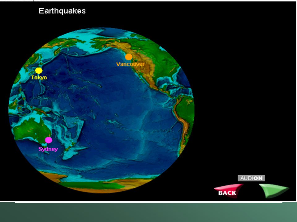
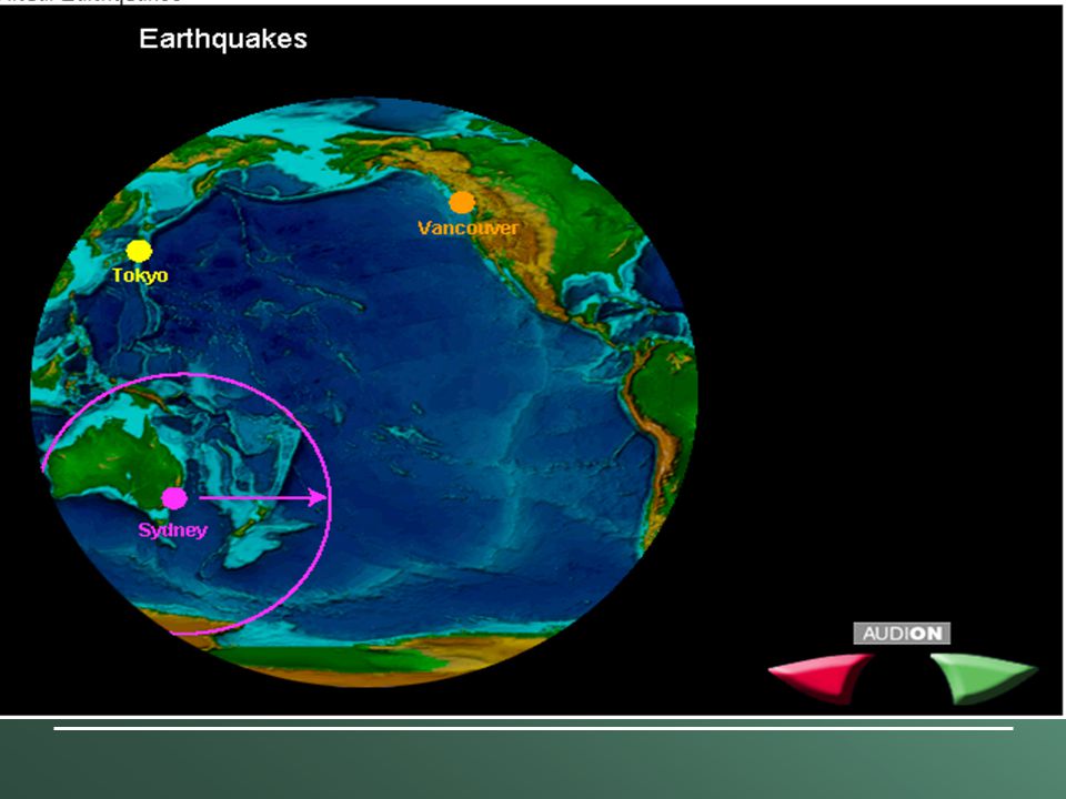
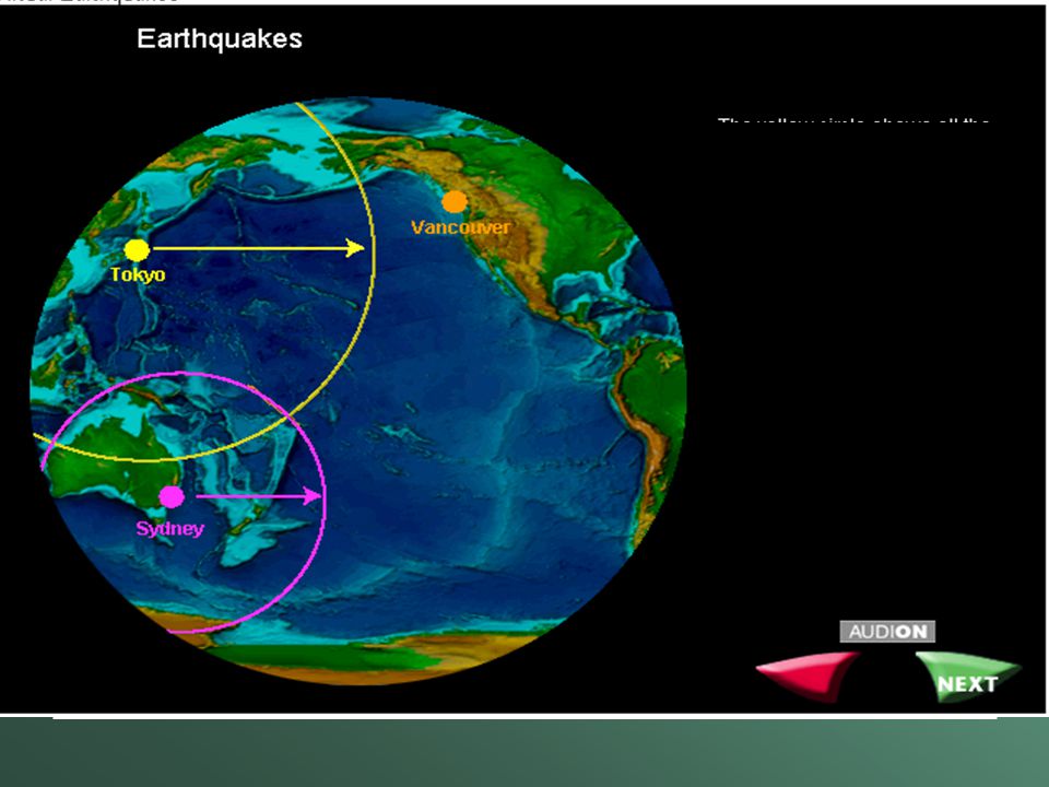
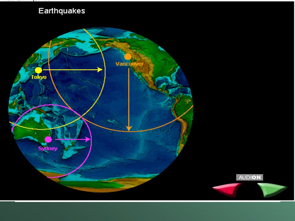
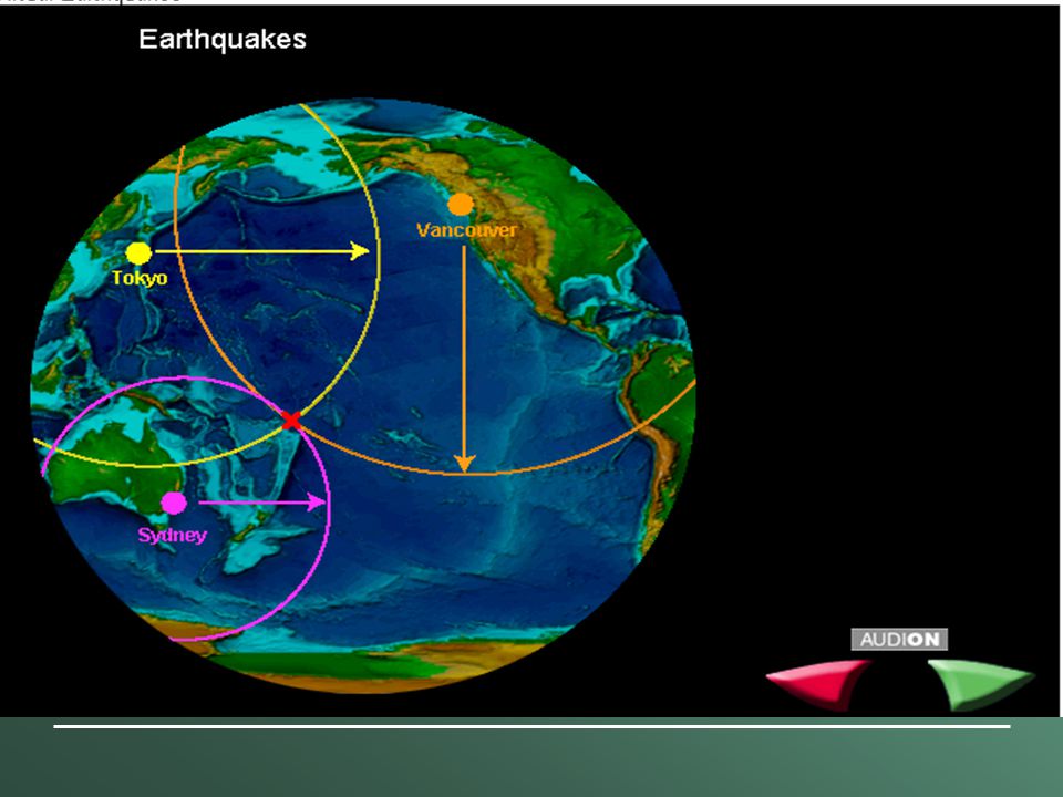
S-P method 1 station – know the distance - a circle of possible location 2 stations – two circles that will intersect at two locations 3 stations – 3 circles, one intersection = unique location With one station the S-P time gives a distance from the station to the source. The earthquake can therefore be anywhere on a circle, centered on the station and with a radius equal to the epicentral distance. With two stations there are two circles and two possible locations. Three stations allow a unique solution to the location. However, additional stations are useful as they reduce any uncorrelated errors (such as picking error). 4+ stations – over determined problem – can get an estimation of errors
. 4+ stations – over determined problem – can get an estimation of errors.")
13
Wadati diagram gives the origin time (where S-P time = 0)
S-P time against absolute P arrival time gives the origin time (where S-P time = 0) Determines Vp/Vs (assuming it’s constant and the P and S phases are the same type – e.g. Pn and Sn, or Pg and Sg) indicates pick errors The Wadati diagram is quite a useful and very simple tool. The S-P time is plotted against the absolute P arrival time. As S-P time goes to zero at the source, by back-projecting the best fit line through the picks we retrieve the origin time of the event. The gradient of the line gives Vp/Vs-1. Here the origin time is ~2 sec past the minute and the gradient is 0.73; therefore Vp/Vs = The exact value of the Vp/Vs ration depends on the composition, temperature, etc of the rocks, so for local earthquakes this is a good independent measure of crustal properties. The points do not fall exactly on the line indicating either that the are variations in the crustal structure (not uniform Vp/Vs) or picking errors, either not being the same type or arrival or misread time.
 Determines Vp/Vs (assuming it’s constant and the P and S phases are the same type – e.g. Pn and Sn, or Pg and Sg) indicates pick errors. The Wadati diagram is quite a useful and very simple tool. The S-P time is plotted against the absolute P arrival time. As S-P time goes to zero at the source, by back-projecting the best fit line through the picks we retrieve the origin time of the event. The gradient of the line gives Vp/Vs-1. Here the origin time is ~2 sec past the minute and the gradient is 0.73; therefore Vp/Vs = The exact value of the Vp/Vs ration depends on the composition, temperature, etc of the rocks, so for local earthquakes this is a good independent measure of crustal properties. The points do not fall exactly on the line indicating either that the are variations in the crustal structure (not uniform Vp/Vs) or picking errors, either not being the same type or arrival or misread time.")
14
Locating with P only The location has 4 unknowns (t,x,y,z) so with 4+ P arrivals this can be solved. The S-P method is easy to understand, but picking S waves accurately is not as easy picking P phases, as there is much more energy on the seismogram from earlier phases. So some location algorithms use only the P phase arrival time to locate the earthquake. This is not as simple as S-P as the relationship between arrival time and distance to the event is non-linear. Therefore it is not particularly easy to solve this problem for the location, and numerical methods are needed. The P arrival time has a non-linear relationship to the location, even in the simplest case when we assume constant velocity – therefore can only be solved numerically

15
Numerical methods tci = T(xi,yi,zi,x0,y0,z0) + t0
Calculated travel time: Simplest possible relation between travel time and location: Find location by minimizing the summed residual (e): tci = T(xi,yi,zi,x0,y0,z0) + t0 ti = √(x0- xi)2+(y0-yi)2 v Can express the calculated travel time (tci) at station “i” as the travel time (T) plus the origin time (t0) where T is a function of the known station location (xi,yi,zi) and the unknown source location (x0,y0,z0) . However, even if the velocity is constant (so the travel time is a simply the distance between the quake and the station divided by the velocity) the travel time is not a linear function of the location. Therefore the location cannot be found analytically, it needs to be calculated by numerical methods. There are many possible ways of finding a numerical solution, we will just discuss some of the more common. But for all methods the central idea is to find a location that minimizes the difference between the calculated (tci) and the observed arrival time (ti). The difference is called the residual. ri is the residual for a single station, the aim is to find a location that minimizes the residual for all stations, so some way is required of comparing the residuals from all stations. The most common approach is to the “least squares” which aims to find the minimize the sum of the squared residuals (e) - squared to remove the canceling effects of having some positive and some negative residuals. Often an ‘average’ station misfit is reported (as this is easier to understand and think about in terms of picking errors, etc then the sum of the residuals), this is commonly the RMS misfit (root mean squared), which is √(e/n) (where n= the number of observations used to calculate e). Note that e (or the RMS squared) is similar but not quite the same as the variance in the data, variance is e/n where n= number of degrees of freedom, which is the number of data – number of parameters in the fit (which is 4 here). n ri = ti – tci e = Σ (ri)2 i=1
: tci = T(xi,yi,zi,x0,y0,z0) + t0. ti = √(x0- xi)2+(y0-yi)2. v. Can express the calculated travel time (tci) at station i as the travel time (T) plus the origin time (t0) where T is a function of the known station location (xi,yi,zi) and the unknown source location (x0,y0,z0) . However, even if the velocity is constant (so the travel time is a simply the distance between the quake and the station divided by the velocity) the travel time is not a linear function of the location. Therefore the location cannot be found analytically, it needs to be calculated by numerical methods. There are many possible ways of finding a numerical solution, we will just discuss some of the more common. But for all methods the central idea is to find a location that minimizes the difference between the calculated (tci) and the observed arrival time (ti). The difference is called the residual. ri is the residual for a single station, the aim is to find a location that minimizes the residual for all stations, so some way is required of comparing the residuals from all stations. The most common approach is to the least squares which aims to find the minimize the sum of the squared residuals (e) - squared to remove the canceling effects of having some positive and some negative residuals. Often an ‘average’ station misfit is reported (as this is easier to understand and think about in terms of picking errors, etc then the sum of the residuals), this is commonly the RMS misfit (root mean squared), which is √(e/n) (where n= the number of observations used to calculate e). Note that e (or the RMS squared) is similar but not quite the same as the variance in the data, variance is e/n where n= number of degrees of freedom, which is the number of data – number of parameters in the fit (which is 4 here). n. ri = ti – tci e = Σ (ri)2. i=1.")
16
Least squares – the outlier problem
The squaring makes the solution very sensitive to outliers. Algorithms normally leave out points with large residuals The least squares approach is simple to compute and is therefore extremely widely used. However, it is quite a fragile optimization and is particularly sensitive to outliers (i.e. data that fall a long way from the main trend). For example a data point with a residual of 1 contributes 1 to the calculation of e, whereas a data point with a residual of 4 contributes 16 to the sum e (i.e. has 16 times more effect). There are other more robust methods of calculating the function that is minimized, such as using the sum of the absolute value of the residual (e = Σ|ri|), which is known as the L1 norm, but these complicate the equations and so are not popular. When dealing with earthquake location, outliers are likely to represent picking mistakes and therefore can cause mislocations. To reduce this effect the location programs normally have a method of weighting the data that affectively removes individual picks with large residuals from the location calculation
. For example a data point with a residual of 1 contributes 1 to the calculation of e, whereas a data point with a residual of 4 contributes 16 to the sum e (i.e. has 16 times more effect). There are other more robust methods of calculating the function that is minimized, such as using the sum of the absolute value of the residual (e = Σ|ri|), which is known as the L1 norm, but these complicate the equations and so are not popular. When dealing with earthquake location, outliers are likely to represent picking mistakes and therefore can cause mislocations. To reduce this effect the location programs normally have a method of weighting the data that affectively removes individual picks with large residuals from the location calculation.")
17
Numerical methods – grid search
As well as a measure of the fit of the location to the data we need a method of choosing a location to test, the simplest way to do this is a grid search, i.e. all locations on a grid are tested and the misfit mapped out, and the earthquake location is (at least in theory) where the minimum misfit is. courtesy of Robert Mereu
 where the minimum misfit is. courtesy of Robert Mereu.")
18
solving using linearization
tci = T(xi,yi,zi,x0,y0,z0) + t0 ri = ti – tci Assume a starting location and assume that the change needed (Δx Δy Δz Δt) is small enough that a Taylor series expansion with only the linear term keep is a good approximation: In reality we rarely use a grid search as it requires a huge number of calculation instead we attempt to “linearize” the problem (i.e. restructure the problem so that the residuals are a linear function of the changes needed to the hypocentral distance). The most common approach is to assume a starting location of the station with the earliest recorded arrival (e.g. the nearest station to the event) and assume that small changes to this location will give the hypocenter. We use the notation Δx Δy Δz Δt to indicate the changes in location and time needed. With this assumption we can use a Taylor series expansion, keeping only the first term. This reduces the relationship between the residual (ri) and the required changes in location to set of linear equations. At the bottom of the slide we have the equation for one station (i). ri = (δT/δxi)Δx + (δT/δyi)Δy + (δT/δzi)Δz + Δt
 + t0. ri = ti – tci. Assume a starting location and assume that the change needed (Δx Δy Δz Δt) is small enough that a Taylor series expansion with only the linear term keep is a good approximation: In reality we rarely use a grid search as it requires a huge number of calculation instead we attempt to linearize the problem (i.e. restructure the problem so that the residuals are a linear function of the changes needed to the hypocentral distance). The most common approach is to assume a starting location of the station with the earliest recorded arrival (e.g. the nearest station to the event) and assume that small changes to this location will give the hypocenter. We use the notation Δx Δy Δz Δt to indicate the changes in location and time needed. With this assumption we can use a Taylor series expansion, keeping only the first term. This reduces the relationship between the residual (ri) and the required changes in location to set of linear equations. At the bottom of the slide we have the equation for one station (i). ri = (δT/δxi)Δx + (δT/δyi)Δy + (δT/δzi)Δz + Δt.")
19
solving using linearization
ri = (δT/δxi)Δx + (δT/δyi)Δy + (δT/δzi)Δz + Δt r = G m In matrix notation: r - the vector of residuals G - the partial derivatives (each entry in the 4th column = 1) m - the correction factor for each variable The equation at the bottom of the last slide can be written in vector notation as r = Gm, where r is the vector containing the residuals for each station (where are easily calculated after and initial guess as the location), G is the matrix of partial derivatives (i.e. Gi1, Gi2, and Gi3 are the dT/dx, dT/dy and dT/dz for station i and Gi4 is always 1, for the partial derivative of the origin time term) and is evaluated from the velocity model (see the next slide), m is the vector of model adjustments, this is what we are solving for.
Δx + (δT/δyi)Δy + (δT/δzi)Δz + Δt. r = G m. In matrix notation: r - the vector of residuals. G - the partial derivatives. (each entry in the 4th. column = 1) m - the correction factor for. each variable. The equation at the bottom of the last slide can be written in vector notation as r = Gm, where r is the vector containing the residuals for each station (where are easily calculated after and initial guess as the location), G is the matrix of partial derivatives (i.e. Gi1, Gi2, and Gi3 are the dT/dx, dT/dy and dT/dz for station i and Gi4 is always 1, for the partial derivative of the origin time term) and is evaluated from the velocity model (see the next slide), m is the vector of model adjustments, this is what we are solving for.")
20
iterative solution Counteract the approximation of linearizing the problem by taking the solution as a new starting model. starting location calc solution true location Having found the model adjustment needed to our first guess we now have a solution. However, we only have the approximate solution as we linearized the problem. So now we take the ‘solution’ and use it as a new starting model as repeat the process. We continue to do this until the there is little change between iterations. Then we assume we have the solution. However we have no idea if we have found the true minima or a local minima in the solution. iteration residual

21
A grid search may show if there is a better solution
The residuals are not always a well behaved function, can have local minima The error measure for the location (e.g. RMS misfit) does not necessarily have a simple shape, instead (as shown in the top right) it can have local minima isolated from the global minima. By checking the area around the solution with a grid search it possible to check whether the function varies smoothly (like the bottom left) or contains other minima. A grid search may show if there is a better solution
 does not necessarily have a simple shape, instead (as shown in the top right) it can have local minima isolated from the global minima. By checking the area around the solution with a grid search it possible to check whether the function varies smoothly (like the bottom left) or contains other minima. A grid search may show if there is a better solution.")
22
Single station method The S-P time give the distance to the epicenter
Particle motion – P wave N The S-P time give the distance to the epicenter The ratio of movement on the horizontal components gives the azimuth Station W E to event S UP With 3 component stations an approximate location can be found from a single station. This is not just an interesting observation, this method can be used to help constrain the search for multi-station location methods. In the example shown here the first P wave particle motion is up (positive on Z), north (positive on N) and west (negative on E) – the combination of northward and westward motion on the horizontals indicates that the event is in either the NW or SE quadrants (see the particle motion map), as the energy must have come through the ground and the first motion is up, N, W, the event must be in the SE quadrant. The particle motion maps also show that by measuring the ratio of movement on the E and N components over a few cycles of the P wave, the azimuth can be estimated to the nearest 20 degrees or so. UP Station W E N to event W DOWN
, north (positive on N) and west (negative on E) – the combination of northward and westward motion on the horizontals indicates that the event is in either the NW or SE quadrants (see the particle motion map), as the energy must have come through the ground and the first motion is up, N, W, the event must be in the SE quadrant. The particle motion maps also show that by measuring the ratio of movement on the E and N components over a few cycles of the P wave, the azimuth can be estimated to the nearest 20 degrees or so. UP. Station. W. E. N. to event. W. DOWN.")
23
Depth estimation ANSS station spacing ~280 km
The distance between the station and the event is likely to be many kilometers. Therefore a small variation in focal depth (e.g. 5 km) will have little effect on the distance between the event and the station. Therefore the S-P time and P arrival time are insensitive to focal depth Knowing the depth of the event important for all applications of earthquake seismology, and especially for tsunami warnings. The tsunami is generated by disturbances in the sea floor, so if the event to too deep to rupture (or significantly deform) the seabed then there is a greatly reduced tsunami risk – there is still a risk of a tsunami generated by a landslide triggered by the ground shaking, but the risk is smaller than for a significant seabed rupture. Therefore it is important to know if the epicenter is 5 km or 50 km depth. Unfortunately the geometry of the stations is likely to make the depth very uncertain if we only have S-P or P arrival times. The station spacing is likely to be several tens of kilometers at best (and for the Indian Ocean at the moment it is more like hundreds of kilometers in most regions). For example, the backbone coverage of the US Advance National Seismic System has a station spacing of roughly 280 km (although the coverage is far greater in high hazard areas, like California, where there is about a 20 km spacing on average). With large station intervals the distance between the quake and the station is very insensitive to the depth of the event. tens to hundreds of kilometers 10 km 20 km
 will have little effect on the distance between the event and the station. Therefore the S-P time and P arrival time are insensitive to focal depth. Knowing the depth of the event important for all applications of earthquake seismology, and especially for tsunami warnings. The tsunami is generated by disturbances in the sea floor, so if the event to too deep to rupture (or significantly deform) the seabed then there is a greatly reduced tsunami risk – there is still a risk of a tsunami generated by a landslide triggered by the ground shaking, but the risk is smaller than for a significant seabed rupture. Therefore it is important to know if the epicenter is 5 km or 50 km depth. Unfortunately the geometry of the stations is likely to make the depth very uncertain if we only have S-P or P arrival times. The station spacing is likely to be several tens of kilometers at best (and for the Indian Ocean at the moment it is more like hundreds of kilometers in most regions). For example, the backbone coverage of the US Advance National Seismic System has a station spacing of roughly 280 km (although the coverage is far greater in high hazard areas, like California, where there is about a 20 km spacing on average). With large station intervals the distance between the quake and the station is very insensitive to the depth of the event. tens to hundreds of kilometers. 10 km. 20 km.")
24
courtesy of Robert Mereu
Synthetic tests of variation in depth resolution - used in designing the network. As the distance for the quake to the nearest station increases the network becomes insensitive to the depth of the event (which was 10km for this test data). These are synthetic tests to illustrate how sensitivity to earthquake depth decreases with distance to the nearest station. When the closest station is less than 10 km from the event the location is very sensitive to the depth of the event, as shown by the high error for solution with different depths to the 10 km of the simulated earthquake. With the nearest station at 25 km, the depth is much more poorly resolved and if the closest station is more then 40 km from the event then there is almost no depth resolution.
. These are synthetic tests to illustrate how sensitivity to earthquake depth decreases with distance to the nearest station. When the closest station is less than 10 km from the event the location is very sensitive to the depth of the event, as shown by the high error for solution with different depths to the 10 km of the simulated earthquake. With the nearest station at 25 km, the depth is much more poorly resolved and if the closest station is more then 40 km from the event then there is almost no depth resolution.")
25
Depth – pP and sP The phases that reflect from the Earth surface near the course (pP and sP) can be used to get a more accurate depth estimate However, because energy is radiated from the source in all directions, for distant events it may be possible to identify a phase that travels up from the source and reflects from the surface of the Earth. If the energy travels as a P wave from the source this arrival is called pP; but energy that leaves the source as an S wave can also be converted to a P when reflected, this arrival is called sP. Almost the only difference in travel path between pP and P (or sP and P) is the path from the focus to the earth surface and back. Therefore, the difference in travel time for P and pP (or P and sP) is controlled by the depth of the source. So this can be used to get a much more accurate depth estimate for events when there isn’t a very local seismic station. Stein and Wysession “An Introduction to Seismology, Earthquakes, and Earth Structure”
 is the path from the focus to the earth surface and back. Therefore, the difference in travel time for P and pP (or P and sP) is controlled by the depth of the source. So this can be used to get a much more accurate depth estimate for events when there isn’t a very local seismic station. Stein and Wysession An Introduction to Seismology, Earthquakes, and Earth Structure")
26
Velocity models For distant events may use a 1-D reference model (e.g. PREM) and station corrections All locations rely on a good velocity model to convert time to distance, so now we’ll look a little more a velocity models. Generally we use a simple 1D velocity model as this allows relatively easy conversion of time to distance, saving computational time. Generally this seems to give adequate locations (with small RMS misfits). For distant events we use a standard reference earth model (e.g. PREM, AK135, ISAP91) which includes the velocity structure of the deep earth. In this slide we see the velocity structure on the left and the distance-time plot this generates on the right.
. For distant events we use a standard reference earth model (e.g. PREM, AK135, ISAP91) which includes the velocity structure of the deep earth. In this slide we see the velocity structure on the left and the distance-time plot this generates on the right.")
27
Local velocity model For local earthquakes need a model that represents the (1D) structure of the local crust. For local earthquakes we usually use a local 1D model of the crust and upper mantle, often with a simple linear gradient and a velocity step at the Moho. The example on this slide is for a Moho depth of 35 km (a little thinner than the global average), a crustal velocity gradient from 5 km/s-6.8 km/s for P waves and an upper mantle P wave velocity of 8. This model would be adjusted for different areas, for example, changing the crustal thickness or allowing for slow sediments at the surface. SeisGram2K
, a crustal velocity gradient from 5 km/s-6.8 km/s for P waves and an upper mantle P wave velocity of 8. This model would be adjusted for different areas, for example, changing the crustal thickness or allowing for slow sediments at the surface. SeisGram2K.")
28
Determining the local velocity model
Refraction data the best for Moho depth and velocity structure of the crust. To determine the local velocity structure we often use controlled source (also called active source) techniques. These are experiments done using controlled sources (explosions or vibrators on land, air gun shots at sea). They use a very dense coverage of either sources or temporary stations and optimize the distribution to look at the structure of the crust. The best method for determining seismic velocity of the crust and upper mantle and the depth of the Moho is the refraction method. However, these experiments are relatively expensive to run and until recently have mostly be done for academic research and so are not always available. Normal incidence reflection methods can also provide information on the velocity of the crust and depth/structure of the Moho, but do not get this information as precisely. But reflection surveying has been done by oil companies over much more extensive areas than refraction surveying (although often for only the upper crust). Winnardhi and Mereu, 1997.
 techniques. These are experiments done using controlled sources (explosions or vibrators on land, air gun shots at sea). They use a very dense coverage of either sources or temporary stations and optimize the distribution to look at the structure of the crust. The best method for determining seismic velocity of the crust and upper mantle and the depth of the Moho is the refraction method. However, these experiments are relatively expensive to run and until recently have mostly be done for academic research and so are not always available. Normal incidence reflection methods can also provide information on the velocity of the crust and depth/structure of the Moho, but do not get this information as precisely. But reflection surveying has been done by oil companies over much more extensive areas than refraction surveying (although often for only the upper crust). Winnardhi and Mereu,")
29
Art Jolly http://www. giseis. alaska
Tomography Local tomography from local earthquakes can give crust and upper mantle velocities Regional/Global tomography from global events gives mantle velocity structure. seismic tomography is the method of mapping out the velocity structure in very well sampled area by looking at the variation in travel time of different paths through the area. Local tomography from local earthquakes or controlled sources can give detailed maps of the crustal velocity, for example the top image is the velocity (at 2-4 km below the surface) around a volcano in Alaska, resolved using the earthquakes from magma movement (black dots) recorded at a number of local stations (black triangles). The lower image is an example of regional seismic tomography done using regional or teleseismic earthquakes. Here we see a very clear variation in seismic velocity associated with the subduction Pacific Plate and melting in the mantle wedge above the plate. We can see that such images can provide very detailed information on the velocity variation, but require a large number of sources and stations and considerable computation, so high resolution local models are not widely available around the globe. Seismic Tomography at the Tonga Arc Zone (Zhao et al., 1994)
 around a volcano in Alaska, resolved using the earthquakes from magma movement (black dots) recorded at a number of local stations (black triangles). The lower image is an example of regional seismic tomography done using regional or teleseismic earthquakes. Here we see a very clear variation in seismic velocity associated with the subduction Pacific Plate and melting in the mantle wedge above the plate. We can see that such images can provide very detailed information on the velocity variation, but require a large number of sources and stations and considerable computation, so high resolution local models are not widely available around the globe. Seismic Tomography at the Tonga Arc Zone. (Zhao et al., 1994)")
30
Contours of the P-wave Station Correction, NE India
Station Corrections Station corrections allow for local structure and differences from the 1D model Contours of the P-wave Station Correction, NE India The many refraction, reflection and tomographic studies around the globe show that the velocity structure of the crust is not a simple 1D model, but has considerable local variation. However, as mentioned earlier, a 1D model is far easier to use in the location calculation. One way of reducing the errors introduced by using a 1D model is to add station corrections. These are effectively a static shift applied to the arrival times at a recording station to account for local differences to the 1D model. For example a station located far above sea level will record delayed arrivals with respect to the 1D model, due to the extra distance the energy is traveling. Or a station on in a sedimentary basin will also have a delay due to the low velocity beneath the seismometer. However, it must be noted that station correction is a constant correction applied to all arrivals (from all distances and directions) and so can only correct for the structure very close to the station, not for deeper structure that will affect only arrivals from a certain distance and azimuth. (Bhattacharya et al., 2005)
 and so can only correct for the structure very close to the station, not for deeper structure that will affect only arrivals from a certain distance and azimuth. (Bhattacharya et al., 2005)")
31
Location in subduction zones
Poor station distribution Good location Locations for tsunami warning centers often face a problem with station distribution. The smallest uncertainties are for events surrounded by stations. When all stations are at a similar azimuth then the location is much more poorly constrained. For shallow subduction zone earthquakes, this is often a problem as the seismometers are normally only deployed on land (only the JMA has ocean bottom seismometers for tsunami warnings) and the geological processes mean the land is almost all on the back arc side of the trench. Therefore, the stations are often all on one side of the earthquake. Poor location
 and the geological processes mean the land is almost all on the back arc side of the trench. Therefore, the stations are often all on one side of the earthquake. Poor location.")
32
Stations in the Indian Ocean
In the Indian Ocean there is a plan to greatly improve the station density, which will hugely improve earthquake location. But the stations will be deployed in numerous countries, and so the success of the tsunami warning system is going to rely on international co-operation and data sharing. Operational Planned Courtesy L. Kong

33
Relocation methods Network locations relocations Recalculate the locations using the relationship between the events. Master Event Method Joint hypocentral determination Double difference method Although there will not be time to use relocation for tsunami warning purposes, it might be possible to analyze events more thoroughly afterwards. In this case, relocation methods might be of interest for better characterizing the source of the earthquakes. One of the main sources of error in the location is error in the velocity model; however if a number of events are very closely spaced (for example microearthquakes on a well instrumented fault, or aftershocks) then the ray paths from the source to the stations will be very similar for all the events. The total travel time for each individual event is subject to any errors in the velocity model, but the difference in travel time between events is related to the spatial distance between the sources. Therefore by comparing events the relative locations can be judged much more accurately than the absolute location. On the examples on the right, we can see that after relocation of events in Northern California the faults appear much sharper and artifacts like the arch of events seen in the original locations are removed. A better map of faults helps to better define the seismic hazard. Waldhauser and Schaff “Improving Earthquake Locations in Northern California Using Waveform Based Differential Time Measurements”
 then the ray paths from the source to the stations will be very similar for all the events. The total travel time for each individual event is subject to any errors in the velocity model, but the difference in travel time between events is related to the spatial distance between the sources. Therefore by comparing events the relative locations can be judged much more accurately than the absolute location. On the examples on the right, we can see that after relocation of events in Northern California the faults appear much sharper and artifacts like the arch of events seen in the original locations are removed. A better map of faults helps to better define the seismic hazard. Waldhauser and Schaff Improving Earthquake Locations in Northern California Using Waveform Based Differential Time Measurements")
34
Master event relocation
Select master event(s) – quakes with good locations, probably either the largest magnitude or event(s) that occurred after a temporary deployment of seismographs. Assign residuals from this event as the station corrections. Relocated other events using these station corrections. Master event relocation can be used to better resolve the relative distribution of a cluster of earthquakes (for example a main shock and the series of after shocks). Such work can be useful for defining the structure of faults or the area that slipped in a large earthquake. The basic idea is to take one of the events that is assumed to have the best location (often the main shock in a main shock-aftershock sequence – as this well have the best signal to noise ratio) and assume that the residual travel time misfits for the best location are due to deviations in the velocity structure. Then because the paths from events in the cluster will be similar for all events, these deviations in velocity model are assumed to be the same for all events. So the arrival times for other events in the cluster are adjusted using the master event residuals, and the events relocated.
 – quakes with good locations, probably either the largest magnitude or event(s) that occurred after a temporary deployment of seismographs. Assign residuals from this event as the station corrections. Relocated other events using these station corrections. Master event relocation can be used to better resolve the relative distribution of a cluster of earthquakes (for example a main shock and the series of after shocks). Such work can be useful for defining the structure of faults or the area that slipped in a large earthquake. The basic idea is to take one of the events that is assumed to have the best location (often the main shock in a main shock-aftershock sequence – as this well have the best signal to noise ratio) and assume that the residual travel time misfits for the best location are due to deviations in the velocity structure. Then because the paths from events in the cluster will be similar for all events, these deviations in velocity model are assumed to be the same for all events. So the arrival times for other events in the cluster are adjusted using the master event residuals, and the events relocated.")
35
Cross-correlation to improve picks
Phases from events with similar locations and focal mechanisms will have similar waveforms. realign traces to maximize the cross-correlation of the waveform. Analyst Picks Cross-correlated Picks If two or more records have similar waveforms (needs similar location and focal mechanism – e.g. a recurring event on the same fault, or recordings on an array) then the time of the phase onset can be very accurately determined by maximizing the cross correlation between the traces – this has been shown to be times more accurate then manual picking of events, but it needs similar waveforms. Rowe et al Pure and Applied Geophysics 159
 then the time of the phase onset can be very accurately determined by maximizing the cross correlation between the traces – this has been shown to be times more accurate then manual picking of events, but it needs similar waveforms. Rowe et al Pure and Applied Geophysics 159.")
36
Some additional related topics...
Waveform modeling Automated phase pickers location of great earthquakes

37
Waveform modeling Generate synthetic waveforms and compare to the recorded data to constrain the event The arrival time is only one piece of data that is available in the seismogram, there is much more data available if we use the whole waveform. To extract this data we construct synthetic seismograms and compare them to the observed waveforms, adjusting the parameters (such as depth of the event) until there is a good agreement between synthetic and observed. The figure (which we’ve already seen) illustrates this for estimating the depth of the event: with a deeper event the separation between P and pP and PwP (reflection from the ocean surface – w for water) increases. On the right we can se how this effects the synthetic seismogram and this shows that 30 km is the best depth for this data. Note that by waveform modeling we can determine the effect of the pP, sP, SwP and PwP phases on the seismogram even when they merge into the P arrival and cannot be easily picked as separate arrivals. Stein and Wysession “An Introduction to Seismology, Earthquakes, and Earth Structure”
 until there is a good agreement between synthetic and observed. The figure (which we’ve already seen) illustrates this for estimating the depth of the event: with a deeper event the separation between P and pP and PwP (reflection from the ocean surface – w for water) increases. On the right we can se how this effects the synthetic seismogram and this shows that 30 km is the best depth for this data. Note that by waveform modeling we can determine the effect of the pP, sP, SwP and PwP phases on the seismogram even when they merge into the P arrival and cannot be easily picked as separate arrivals. Stein and Wysession An Introduction to Seismology, Earthquakes, and Earth Structure")
38
u(t) = x(t) * e(t) * q(t) * i(t) U(ω)= X(ω) E(ω) Q(ω) I(ω)
Waveform modeling Construction of the synthetic seismogram u(t) = x(t) * e(t) * q(t) * i(t) seismogram source time function instrument response reflections & conversions at interfaces attenuation U(ω)= X(ω) E(ω) Q(ω) I(ω) We will talk more about how waveform modeling is done in the lecture on focal mechanisms. But the basic idea is that the recorded seismogram is the source function (the signal from the earthquake) modified by it’s path through the Earth and the imperfect response from the instrument. The effect of the path through the Earth is here divided into two components: e(t) is the effect or reflections and conversions at interfaces and q(t) is the attenuation affect (the loss of energy through conversion to heat). Each of these factors works as a convolution (*) in the time domain (or multiplication in the frequency domain).
 = x(t) * e(t) * q(t) * i(t) seismogram. source time function. instrument response. reflections & conversions at interfaces. attenuation. U(ω)= X(ω) E(ω) Q(ω) I(ω) We will talk more about how waveform modeling is done in the lecture on focal mechanisms. But the basic idea is that the recorded seismogram is the source function (the signal from the earthquake) modified by it’s path through the Earth and the imperfect response from the instrument. The effect of the path through the Earth is here divided into two components: e(t) is the effect or reflections and conversions at interfaces and q(t) is the attenuation affect (the loss of energy through conversion to heat). Each of these factors works as a convolution (*) in the time domain (or multiplication in the frequency domain).")
39
Automatic phase picks Short term average - long term average (STA/LTA) – developed in the 1970s, still used by Earthworm and Sac2000 The oldest approach to automated phase picking is the STA/LTA method, which is similar to event detection methods. The event is found by comparing short term “characteristic function” (CV) to predicted value (PV) based on longer term analysis and the previous analysis. If the CV is greater than the PV multiplied by some threshold value then an event is detected. The CV can be as simple as the absolute magnitude of the seismogram, but is generally something that combines amplitude and frequency. This approach is still widely used for event detection, for example at the HGN station in the Netherlands event detection is done using a STA/LTA algorithm with STA=1 sec, LTA=30 sec, and threshold 8) Sleeman and von Eck 1999, Physics of Earth and Planetary Interiors 113
 to predicted value (PV) based on longer term analysis and the previous analysis. If the CV is greater than the PV multiplied by some threshold value then an event is detected. The CV can be as simple as the absolute magnitude of the seismogram, but is generally something that combines amplitude and frequency. This approach is still widely used for event detection, for example at the HGN station in the Netherlands event detection is done using a STA/LTA algorithm with STA=1 sec, LTA=30 sec, and threshold 8) Sleeman and von Eck 1999, Physics of Earth and Planetary Interiors 113.")
40
Location of Great Earthquakes
With great earthquakes the slip area is very large (hundreds of kilometers) For hazard assessment the epicenter and centroid are not very informative. Need to rupture area, but this is not available in time for tsunami warnings/disaster management. Just a final point, with great quakes the slip zone will be very large, for example ~1200km long for Sumatra So for hazard assessment, tsunami warning and disaster response, we’d really like to know the distribution of the slip and the size and location of the whole rupture. Unfortunately, this is not currently available for many days. What we get is the epicenter from p-wave arrival time, or the centroid (effectively the center of the rupture) from moment tensor inversion. If we look at the great Sumatra earthquake of 2004, we can see how important the difference between these three descriptions is: the rupture propagated north for ~1200 km and so the epicenter and centroid are a very long way from some of the rupture zones, and it seems that the main tsunamigenic portion of the rupture was approximately the central third, not the zone near to the epicenter. This must be remembered when considering tsunami arrival times – the central third is significantly closer to many of the effected countries and there is less shelter for countries to the east. Had the rupture propagated south rather than north the devastation would have been distributed very differently, but there is currently no way knowing the distribution of slip in the first few minutes. Epicenter Centroid Lay et al 2006, Science 308
 For hazard assessment the epicenter and centroid are not very informative. Need to rupture area, but this is not available in time for tsunami warnings/disaster management. Just a final point, with great quakes the slip zone will be very large, for example ~1200km long for Sumatra So for hazard assessment, tsunami warning and disaster response, we’d really like to know the distribution of the slip and the size and location of the whole rupture. Unfortunately, this is not currently available for many days. What we get is the epicenter from p-wave arrival time, or the centroid (effectively the center of the rupture) from moment tensor inversion. If we look at the great Sumatra earthquake of 2004, we can see how important the difference between these three descriptions is: the rupture propagated north for ~1200 km and so the epicenter and centroid are a very long way from some of the rupture zones, and it seems that the main tsunamigenic portion of the rupture was approximately the central third, not the zone near to the epicenter. This must be remembered when considering tsunami arrival times – the central third is significantly closer to many of the effected countries and there is less shelter for countries to the east. Had the rupture propagated south rather than north the devastation would have been distributed very differently, but there is currently no way knowing the distribution of slip in the first few minutes. Epicenter. Centroid. Lay et al 2006, Science 308.")
Similar presentations

>")


, P. Papadimitriou (1), K. Makropoulos.>")


>")


