1. Introduction to Microarray Data Analysis BMI/IBGP 730 Kun Huang Department of Biomedical Informatics The Ohio State University Autumn 2010

2.  Introduction to gene expression microarray  A middle-man’s approach  Applications of microarray  Microarray data processing/analysis workflow  Data format and visualization  Data normalization  Two-color array  Affymetrix array  Software and databases

3. Review of Biology mRNA, cDNA, exon, intron

4. What is microarray?  If we can assay every single molecule of DNA/RNA of interest directly, do we still need microarray?  Currently direct single-molecule sequencing is still not mature, probes are used instead. Probe is a “middle-man”.

5. How is microarray manufactured? Affymetrix GeneChip silicon chip oligonucleiotide probes lithographically synthesized on the array cRNA is used instead of cDNA

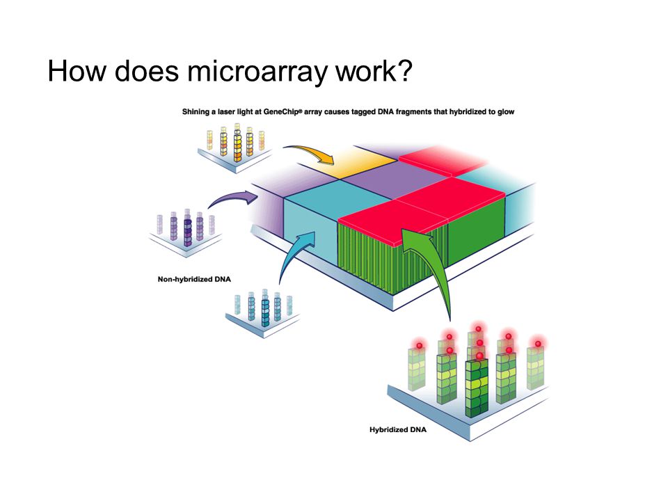
6. How does microarray work?

8. Two-major types of microarray  Affymetrix-like arrays – single channel (background-green, foreground-red)  cDNA arrays – two channel (red, green, yellow)

9. Affymetrix GeneChip  silicon chip  oligonucleiotide probes lithographically synthesized on the array  cRNA is used instead of cDNA

10. Affymetrix GeneChip  silicon chip  oligonucleiotide probes lithographically synthesized on the array

11. Two-channel microarray  Printed microarrays  Long probe oligonucleotides (80-100) long are “printed” on the glass chip  Comparative hybridization experiment

12. Probe selection  Protocol for extracting mRNA  3’ bias – why? Think degradation.  Multiple probes for one region  G-C content http://www.bcgsc.ca/people/malachig/htdocs/alexa_platform/alexa_arrays/intro.htm

13. How do we process microarray data (measurement)?  cDNA array – ratio, log ratio  Affymetrix array

14. Applications of microarrays Gene expression Exon expression SNP detection Copy number variance (arrayCGH) Tiling array (e.g., ChIP-chip)

15. Major vendors Affymetrix Agilent Illumina Nimblegen

16.  Introduction to gene expression microarray  A middle-man’s approach  Applications of microarray  Microarray data processing/analysis workflow  Data format and visualization  Data normalization  Two-color array  Affymetrix array  Software and databases

17. Typical workflow QC Normalization Visualization (boxplot, PCA, RI plot, etc). Comparative study (volcano plot) Clustering Network/pathway inference Motif finding

18. Spatial Images of the Microarrays Data for the same brain voxel but for the untreated control mouse Background levels are much higher than those for the Parkinson’s disearse model mouse There appears to be something non random affecting the background of the green channel of this slide

19. Take a look … (McShane, NCI)

20. Example – Affymetrix Data Files Image file (.dat file) Probe results file (.cel file) Library file (.cdf,.gin files) Results file (.chp file)

21. Example – Affymetrix Data Files Image file (.dat file) Probe results file (.cel file)

22. Scatter plots of the Microarrays A measure of the actual expression levels, i.e., differences between the median foreground and the median background for the red channel and green channel: "F635 Median - B635" "F532 Median - B532” Slope = 1

23. RI plots of the Microarrays RI (ratio-intensity) plot or MA plot

24. Scatter plots of the Microarrays (McShane, NCI)

25. Box plot Median Low quartile Upper quartile

26. Example:

27. Normalization – microarray data is highly noisy  Intensity imbalance between RNA samples  Affect all genes  Not due to biology of samples, but due to technical reasons  Reasons include difference in the settings of the photodetector voltage, imbalance in total amount of RNA in each sample, difference in uptaking of the dyes, etc.  The objective is is to adjust the gene expression values of all genes so that the ones that are not really differentially expressed have similar values across the array(s).

28. Two major issues to consider  Which genes to use for normalization  Which normalization algorithm to use

29. Which genes to use for normalization  Housekeeping genes  Genes involved in essential activities of cell maintenance and survival, but not in cell function and proliferation  These genes will be similarly expressed in all samples.  Difficult to identify – need to be confirmed  Affymetrix GeneChip provides a set of house keeping genes based on a large set of tests on different tissues and were found to have low variability in these samples (but still no guarantee).

30. Which genes to use for normalization  Spiked controls  Genes that are not usually found in the samples (both control and test sample). E.g., yeast gene in human tissue samples.

31. Which genes to use for normalization  Using all genes  Simplest approach – use all adequately expressed genes for normalization  The assumption is that the majority of genes on the array are housekeeping genes and the proportion of over expressed genes is similar to that of the under expressed genes.  If the genes on the chip are specially selected, then this method will not work.

32. Two-color array normalization  Intra-slide normalization  Inter-slide for cDNA arrays

33. Normalization  Linear (global) normalization  Simplest but most consistent  Move the median to zero (slope 1 in scatter plot, this only changes the intersection)  No clear nonliearity or slope in MA plot Slope = 1

34. Normalization  Intensity-based (Loess/Lowess) normalization  Loess/Lowess fit  Overall magnitude of the spot intensity has an impact on the relative intensity between the channels. (McShane, NCI)

35. Normalization  Intensity-based normalization  “Straighten” the Lo(w)ess fit line in MA plot to horizontal line and move it to zero

36. Normalization  Intensity-based (Lowess) normalization  Nonlinear  Gene-by-gene, could introduce bias  Use only when there is a compelling reason (McShane, NCI)

37. Normalization  Quantile normalization  Nonlinear  Same intensity distribution After Lowess normalization After quantile normalization

38. Normalization  Location-based normalization  Background subtracted ratios on the array may vary in a predicable manner.  Sample uniformly across the chip  Nonlinear  Gene-by-gene, could introduce bias  Use only when there is a compelling reason  Other normalization method  Combination of location and intensity-based normalization

39. Normalization  Which normalization algorithm to use  Inter-slide normalization  Not just for Affymetrix arrays

40. Normalization  Linear (global) – the chips have equal median (or mean) intensity  Intensity-based (Lowess) – the chips have equal medians (means) at all intensity values  Quantile – the chips have identical intensity distribution  Quantile is the “best” in term of normalizing the data to desired distribution, however it also changes the gene expression level individually  Potential issues - overfitting

41. Affymetrix array normalization  Inter-slide normalization only  Probe-level normalization  Affymetrix MicroArray Suite (MAS) 5.0  Robust Multiarray Average (RMA)  Quantile  GC-RMA

42. Affymetrix array normalization  Inter-slide normalization only  Probe-level normalization  Affymetrix MicroArray Suite (MAS) 4.0  Simple subtraction of MM from PM  Use only probes within 3 times of SD of PM-MM to exclude outliers  Not robust  MAS 5.0  Use weight (Turkey Biweight Estimate) for each probe based on its intensity difference from the mean  Log transformed data for mean (geometric mean)  Robust

43. Affymetrix array normalization  Robust Multiarray Average (RMA)  Background correction on each chip.  Assuming strictly positive distribution. No negative numbers  Do NOT use MM information  Normalization (inter-chip).  Quantile  Probe level intensity calculation.  Linear model for signal, affinity, and noise.  Probe set summarization.  Combine probes for one probeset into a single number  Median polishing (chip to its median, gene to its median, iterate and converge)

44. Affymetrix array normalization  GC-Robust Multiarray Average (GC-RMA)  Correct back ground noise and non-specific binding  Affinity computed from position specific base effect  MM information is used (subtracted from PM after correction)

45. Affymetrix array normalization  RMA/GCRMA pros and cons (comparing to MAS5.0)  Less variance at low expression values  Less false positives  Consistent fold change estimates  More false negatives, especially for low- expression level probes  Quality control after normalization is difficulty  Quantile normalization may overfit and hide real differences

46.  Introduction to gene expression microarray  A middle-man’s approach  Applications of microarray  Microarray data processing/analysis workflow  Data format and visualization  Data normalization  Two-color array  Affymetrix array  Software and databases

47. Microarray analysis software  Open source R  Bioconductor  BRBArray tools (NCI biometric research branch)  Matlab Bioinformatics Toolbox  Affymetrix Expression Console  DChip  GeneSpring  Partek  …

48. Microarray Databases  Gene Expression Ominbus (GEO) database – NCBI  http://www.ncbi.nlm.nih.gov/entrez/query.fcgi?DB=pubmed  EMBL-EBI microarray database (ArrayExpress)  http://www.ebi.ac.uk/Databases/microarray.html http://www.ebi.ac.uk/Databases/microarray.html  Stanford Microarray Database (SMD)  http://genome-www5.stanford.edu/ http://genome-www5.stanford.edu/  caARRAY sites  The Cancer Genome Atlas (TCGA)  Other specialized, regional and aggregated databases  http://psi081.ba.ars.usda.gov/SGMD/  http://www.oncomine.org/main/index.jsp http://www.oncomine.org/main/index.jsp  http://ihome.cuhk.edu.hk/~b400559/arraysoft_public.html http://ihome.cuhk.edu.hk/~b400559/arraysoft_public.html  …

49.  http://www.ncbi.nlm.nih.gov/projects/geo/query/browse.cgi Gene Expression Omnibus (GEO) Oct. 2006 Oct. 2010

50. Gene Expression Omnibus (GEO)  GEO Profiles This database stores individual gene expression and molecular abundance profiles assembled from the Gene Expression Omnibus (GEO) repository. Search for specific profiles of interest based on gene annotation or pre-computed profile characteristics. GEO Profiles facilitates powerful searching and linking to additional information sources.Gene Expression Omnibus (GEO)  GEO DataSets This database stores curated gene expression and molecular abundance DataSets assembled from the Gene Expression Omnibus (GEO) repository. Enter search terms to locate experiments of interest. DataSet records contain additional resources including cluster tools and differential expression queries.Gene Expression Omnibus (GEO) repository (From GEO website)

51.  GPL  A Platform record describes the list of elements on the array (e.g., cDNAs, oligonucleotide probesets, ORFs, antibodies) or the list of elements that may be detected and quantified in that experiment (e.g., SAGE tags, peptides). Each Platform record is assigned a unique and stable GEO accession number (GPLxxx). A Platform may reference many Samples that have been submitted by multiple submitters.  GSM  A Sample record describes the conditions under which an individual Sample was handled, the manipulations it underwent, and the abundance measurement of each element derived from it. Each Sample record is assigned a unique and stable GEO accession number (GSMxxx). A Sample entity must reference only one Platform and may be included in multiple Series. Gene Expression Omnibus (GEO)

52.  GSE  A Series record defines a set of related Samples considered to be part of a group, how the Samples are related, and if and how they are ordered. A Series provides a focal point and description of the experiment as a whole. Series records may also contain tables describing extracted data, summary conclusions, or analyses. Each Series record is assigned a unique and stable GEO accession number (GSExxx).  GDS  GEO DataSets (GDS) are curated sets of GEO Sample data. A GDS record represents a collection of biologically and statistically comparable GEO Samples and forms the basis of GEO's suite of data display and analysis tools. Samples within a GDS refer to the same Platform, that is, they share a common set of probe elements. Value measurements for each Sample within a GDS are assumed to be calculated in an equivalent manner, that is, considerations such as background processing and normalization are consistent across the dataset. Information reflecting experimental design is provided through GDS subsets. data display and analysis tools Gene Expression Omnibus (GEO)

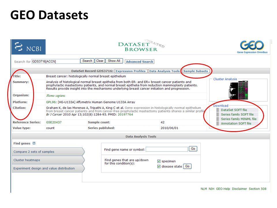
53. GEO Datasets

55. GEO Profiles Number of probesets

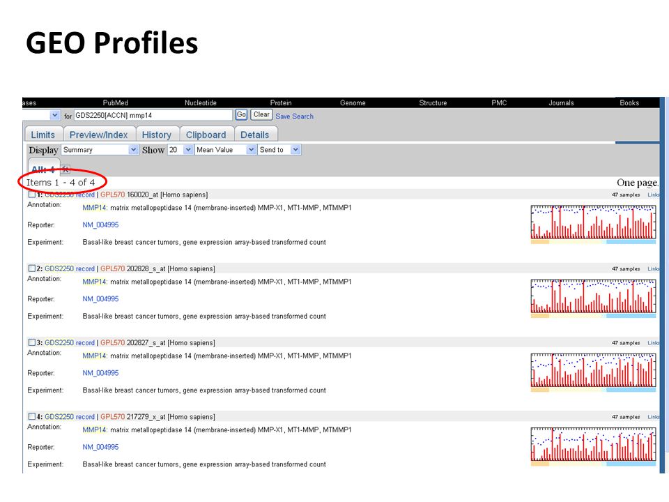
56. GEO Profiles

57. Left y-axis is (supposed to be) log two based (must check to verify) expression level. Right y-axis is the percentile of this expression level in the entire chip. All the chips are normalized. GEO Profiles

59. Multiple probesets for different genes The number of probesets are different Probesets may have different versions May corresponding to polymorphism (splice variants) The results from different probesets may be inconsistent Various ways of combining the data GEO Profiles

60.  Most new datasets are deposited as GSE series datasets instead of GDS datasets and cannot be visualized directly.  Users need to download them for further processing.  A simple way is to download the Data Matrix. GEO Profiles

61. How do we use microarray?  Profiling  Comparative study  Clustering  Network inference

62. Moving beyond microarray?  Cut the middleman  Next generation sequencing  Single-molecule sequencing  Where will microarray go?  Diagnosis  Specialized quick testing kit